10
Object-Oriented Programming and PVector

Object-oriented programming (OOP) deals with data structures known as objects. You create new objects from a class, and you can think of a class as an object template, composed of a collection of related functions and variables. You define a class for each category of objects you want to work with, and each new object will automatically adopt the features you define in its class. OOP combines everything you’ve learned so far, including variables, conditional statements, lists, dictionaries, and functions. OOP adds a remarkably effective way to organize your programs by modeling real-world objects.
You can use classes to model tangible objects, like buildings, people, cats, and cars. Or, you can use them to model more abstract things, like bank accounts, personalities, and physical forces. Although a class will define the general features of a category of objects, you can assign unique attributes to differentiate each object you create. In this chapter, you’ll apply OOP techniques to program an amoeba simulation. You’ll learn how to define an amoeba class, and how to “spawn” varied amoeba from it.
You’ll program amoeba movement by simulating physical forces. For this, you’ll use a built-in Processing class named PVector. The PVector class is an implementation of Euclidean vectors that includes a suite of methods for performing mathematical operations, which you’ll use to calculate the position and movement of each amoeba.
To better manage your code, you’ll learn how to split your program into multiple files. You can then switch between the files that make up your sketch by using tabs in the Processing editor.
Working with Classes
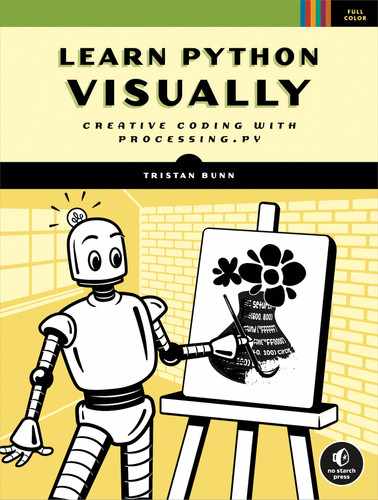
A class is like a blueprint for an object. As an example, consider a Car class that might specify, by default, that all cars have four wheels, a windshield, and so on. Certain features, like the paint color, can vary among individual cars, so when you create a new car object by using the Car class, you get to select a color. Such features are called attributes. In Python, attributes are variables that belong to a class. You can decide which attributes have predefined values (the four wheels and windshield) and which are assigned when you create a new car (the paint color).
In this way, you can create multiple cars, each a different color, using a single class. Figure 10-1 illustrates this concept. The Car class includes attributes to describe the paint color, engine type, and model of each car.
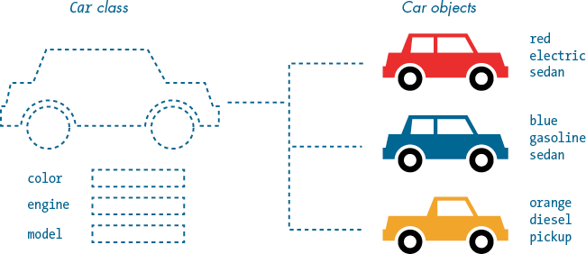
Figure 10-1: The Car class serves as a blueprint for car objects.
Drivers control a vehicle by steering, accelerating, and braking. So in addition to attributes, your Car class can include definitions for performing those actions, referred to as methods. In Python, methods are functions that belong to a class that define the operations or activities it can perform.
Now, let’s define an Amoeba class that includes a set of attributes and methods for controlling the appearance and behavior of amoeba objects. You’ll use that class to create many amoebas. Figure 10-2 depicts the final result of the amoeba simulation that you’re working toward.

Figure 10-2: A screenshot of the complete amoeba simulation
The amoebas will wobble and distort as they move about the display window. This is not a scientifically correct representation of amoebas, but it should look pretty cool. As an extra challenge, you’ll add collision-detection code to prevent them from passing over or through one another. You’ll begin with a basic Amoeba class definition, and then add attributes and methods as you progress through the task.
Defining a New Class
In Python, you define a class by using the class keyword. You may name a class whatever you like, but as with variable and function names, you’re limited to alphanumeric and underscore characters. Because you cannot use space characters, the recommended naming convention for classes is UpperCamelCase, in which the first letter of each word begins with a capital letter, starting with the first word.
To begin, your Amoeba class won’t do much else than print a line to the console. Start a new sketch and save it as microscopic. Define a new Amoeba class:
class Amoeba(object):

    def __init__(self):
        print('amoeba initialized')
The class keyword defines a new class. Here the class name is Amoeba, and it’s followed by object in parentheses, and a colon.
If you run the sketch, nothing interesting should happen, and the console will be empty.
Functions that you define within the body of a class are referred to as methods. The Amoeba class includes a definition for a special method named __init__ (with two underscores at either end). This method is one of a selection of magic methods that start and end with two underscores that you won’t invoke directly. I’ll get into more detail about the __init__() method (and the self parameter) soon. For now, all you need to know is that Python runs the __init__() method automatically for each new amoeba you create. You use this method to set up your attributes and execute code at the time of object creation.
Creating an Instance from a Class
To instantiate an amoeba, you call the Amoeba class by name and assign it to a variable—as you would a function that returns a value. Instantiate is a fancy way of saying create a new instance, and an instance is synonymous with object.
Add a line to create a new instance from your Amoeba class and assign it to a variable named a1:
class Amoeba(object):

    def __init__(self):
        print('amoeba initialized')

a1 = Amoeba()
When you run the sketch, Python creates a new Amoeba() instance. This will automatically invoke the __init__() method. You can use the __init__() method to define attributes and assign values to them, which you’ll do shortly. This method can also include other instructions to initialize the amoeba, as in this case, a print() function. When you run the sketch, the console should display a single amoeba initialized message.
Adding Attributes to a Class
You can think of attributes as variables that belong to an object. And just like a variable, an attribute can contain any data you like, including numbers, strings, lists, dictionaries, and even other objects. For example, a Car class might have a string attribute for the model name and an integer attribute for top speed.
In your Amoeba class, you’ll add three attributes to hold numbers for an x-coordinate, y-coordinate, and diameter; you’ll assign values to those attributes when you instantiate the new amoeba. The syntax resembles that used to pass arguments to a function: the parentheses of the __init__() method contain your list of corresponding parameters.
Make the following changes to your code to accommodate an x, y, and diameter value for each new amoeba:
class Amoeba(object):

    def __init__(self, x, y, diameter):
        print('amoeba initialized')

a1 = Amoeba(400, 200, 100)
The __init__() method already includes a parameter, self; this is required, and it’s always the first parameter. The self parameter provides access to instance-specific values, like an x value of 400 for amoeba a1 (but more on how that works shortly). The x, y, and diameter are added as the second, third, and fourth parameters. I’ve added corresponding arguments to the a1 line. Notice, however, that I provide only three arguments and nothing for the self parameter. Figure 10-3 depicts how these positional arguments match up, starting from the second parameter in the __init__() method.

Figure 10-3: Don’t provide an argument for the self parameter.
You can also use keyword arguments (and specify default values for parameters), but I’ll stick to positional arguments throughout this task.
When you pass values to your __init__() method, it won’t automatically store them for you. For this, you need attributes, which are like variables for objects. Assign the x, y, and diameter parameters to new attributes. Each attribute begins with a prefix of self, followed by a dot, then the attribute name:
class Amoeba(object):

    def __init__(self, x, y, diameter):
        print('amoeba initialized')
        self.x = x
        self.y = y
        self.d = diameter

a1 = Amoeba(400, 200, 100)
Notice that you assign diameter to self.d. Your attribute names need not match your parameter names.
At this point, I can explain more about the self parameter. I’ve mentioned that self is an instance-specific reference. In other words, the self.d value of 100 belongs to amoeba a1. Each amoeba instance will possess its own set of self.x, self.y, and self.d values. For example, I might add another amoeba, a3, with different values:
a3 = Amoeba(600, 250, 200)This will come in handy later when you add multiple amoebas to the simulation. Figure 10-4 provides a conceptual diagram of your Amoeba class and three possible instances.
Next, you’ll learn how to access the x, y, and d values for amoeba a1 via the a1 instance. You’ll use those values to draw the amoeba in the display window, resembling the one depicted in the upper right corner of Figure 10-4.

Figure 10-4: Your Amoeba class and three instances
Accessing Attributes
To access attributes, you use dot notation. For the a1 instance, you can access the x, y, and d attributes as a1.x, a1.y, and a1.d, respectively. This is the instance name (a1) followed by a dot, followed by the name of the attribute you want to access.
To get started, add this code to the end of your sketch, which draws a circle to represent amoeba a1:
. . .
def setup():
    size(800, 400)
    frameRate(120)

def draw():
    background('#004477')
    # cell membrane
    fill(0x880099FF)
    stroke('#FFFFFF')
    strokeWeight(3)
    circle(a1.x, a1.y, a1.d)
The display window is now 800 pixels wide by 400 pixels high. The high frame rate of 120 will help smooth the wobble animation you’ll add to your amoeba later. A cell membrane separates an amoeba’s interior from its outside environment, and here, I’ve given this a white stroke. The fill is a semi-opaque pale blue. For the x-coordinate (first argument) in the circle() function, Python checks the a1 instance for the attribute self.x—in this case, it’s equal to 400; the y-coordinate argument is equal to 200, and the diameter argument is equal to 100. The result (Figure 10-5) is a circle with a diameter of 100 pixels positioned in the center of the display window.

Figure 10-5: A circle (rudimentary amoeba) with a diameter of 100 pixels
So far, you’ve learned how to add arguments to your Amoeba class, which you assign to attributes when you instantiate an amoeba. In addition to those, your class can include attributes with predefined values.
Adding an Attribute with a Default Value
Think back to the car analogy. Every car rolls off the production line with an empty gas tank. The manufacturer may fill it before it’s sold, but the tank always starts empty. For this, you decide to add an attribute to the Car class—let’s call it self.fuel. It has a predefined value of 0 for each new car object, but it’ll fluctuate over the lifetime of the vehicle. It’s redundant to specify by way of an argument that this should start at 0; instead, the Car class should automatically initialize the fuel attribute for you, setting it to 0 by default.
Let’s return to the amoeba task. Every amoeba will include a nucleus with a predefined fill of red. To program this, assign a hexadecimal value (#FF0000) to an attribute named nucleus within the body of your __init__() method. There’s no need to add another parameter to your __init__() definition, because you don’t require the additional argument to specify the red fill:
        . . .
        self.x = x
        self.y = y
        self.d =  diameter
        self.nucleus = '#FF0000'
. . .
Now, every amoeba you create has a nucleus attribute assigned a value of #FF0000.
Insert three new lines in your draw() function to render the nucleus beneath the cell membrane:
. . .
def draw():
    background('#004477')
    # nucleus
    fill(a1.nucleus)
    noStroke()
    circle(a1.x, a1.y, a1.d/2.5)
    # cell membrane
    . . .
The new lines set the fill and stroke, and then draw the nucleus by using a circle() function with a diameter that’s 2.5 times smaller (a1.d/2.5) than that of the cell membrane, placing it in the center of the amoeba. Run the sketch to confirm that you see a mauve nucleus; it is technically red, but you see it through the pale blue, semi-opaque membrane.
You don’t set the nucleus fill when you instantiate the amoeba, but that doesn’t mean you’re stuck with a red nucleus. You can modify the attribute values after you’ve created an amoeba.
Modifying an Attribute Value
Many attributes hold values that change as your program runs. To return to the car analogy, consider the fuel attribute mentioned previously with a value that’s continually shifting as the gas tank fluctuates between full and empty. You can modify the value of any attribute directly via the instance by using the same dot syntax for accessing values.
Insert a line to change the nucleus fill for amoeba instance a1:
    . . .
    # nucleus
    a1.nucleus = '#00FF00'
    fill(a1.nucleus)
    . . .
This sets the nucleus attribute to green, overwriting the default value of red. Run the sketch to confirm that you see a green nucleus showing through the semi-opaque membrane.
You can also modify an attribute by using a method, which I cover in “Adding Methods to a Class” on page 216.
Using a Dictionary for an Attribute
Recall that attributes can contain anything you like—numbers, strings, lists, dictionaries, objects, and so on. You’ll use a dictionary attribute that holds a mix of string (hexadecimal) and floating-point values to group the nucleus properties.
Change your nucleus attribute to a dictionary that holds key-value pairs for a nucleus fill, x-coordinate, y-coordinate, and diameter. To vary the appearance of each amoeba, randomize those values:
class Amoeba(object):

    def __init__(self, x, y, diameter):
        print('amoeba initialized')
        self.x = x
        self.y = y
        self.d = diameter
        self.nucleus = {
          'fill': ['#FF0000', '#FF9900', '#FFFF00',
                   '#00FF00', '#0099FF'][int(random(5))],
          'x': self.d * random(-0.15, 0.15),
          'y': self.d * random(-0.15, 0.15),
          'd': self.d / random(2.5, 4)
        }
. . .
The fill key is paired with a hexadecimal value arbitrarily selected from a list of five colors. The nucleus color of each new amoeba is now chosen at random (although you may explicitly overwrite it afterward). The x and y keys are assigned randomized values proportional to the diameter of the cell membrane; you’ll use those to position the nucleus somewhere within the boundary of the cell membrane, but not necessarily in the center. The diameter of the nucleus (d) is also proportional to the cell membrane and randomly varies for each instance.
Update your draw() code to work with these changes:
. . .
def draw():
    background('#004477')
    # nucleus
    fill(a1.nucleus['fill'])
    noStroke()
    circle(
      a1.x + a1.nucleus['x'],
      a1.y + a1.nucleus['y'],
      a1.nucleus['d']
    )
    # cell membrane
    . . .
The fill() and circle() arguments reference the relevant dictionary keys to style and position the nucleus.
Each time you run the sketch, Processing will generate a unique amoeba. Figure 10-6 depicts four results from four runs. Of course, it’s possible (but unlikely) that Processing will produce the same or a similar selection of randomized values, and consecutive results might appear identical.
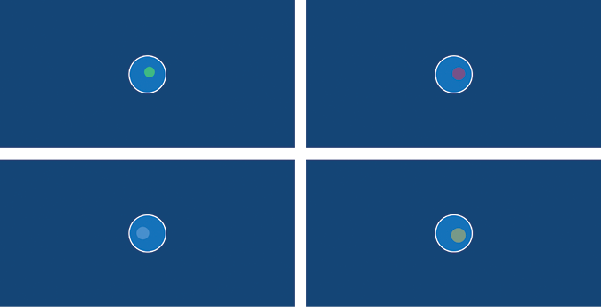
Figure 10-6: Each amoeba is generated using randomized nucleus values.
Now that you’ve set up the attributes to control the visual appearance of your amoeba, the next step is to add methods to animate it.
Adding Methods to a Class
Functions that you define within the body of a class are referred to as methods. To return to the car analogy, drivers can control a vehicle by using methods, such as steering, accelerating, and braking. You could also include a method for refueling. Methods typically perform operations by using an object’s attributes. For example, an accelerate() and refuel() method will subtract from and add to a fuel attribute.
You can name methods whatever you like, as long as you apply the same naming rules and conventions for functions. In other words, use only alphanumeric and underscore characters, camelCase or underscores instead of spaces, and so forth.
You’ll create a new method to draw your amoeba for each frame. Currently, several lines in the draw() section of your code handle this operation. Move the nucleus and cell membrane code from the draw() function into the body of a new display() method, ensuring that your indentation is correct. Replace every a1 prefix with self in the display() method:
class Amoeba(object):
    . . .
    def display(self1):
        # nucleus
        fill(self.nucleus['fill'])
        noStroke()
        circle(
          self.x + self.nucleus['x'],
          self.y + self.nucleus['y'],
          self.nucleus['d']
        )
        # cell membrane
        fill(0x880099FF)
        stroke('#FFFFFF')
        strokeWeight(3)
        circle(self.x, self.y, self.d)
. . .
def draw():
    background('#004477')
The self parameter in the definition 1 provides the body of your display() method with access to your attributes, such as self.nucleus and self.x. The display() method accepts zero arguments, so the definition includes no further parameters.
Calling a Method
Once you’ve defined a method, you can use the same dot notation as for attributes to call the method and execute the code in that method’s body—that is, the instance name followed by the method, separated by a dot. Of course, methods, like functions, include parentheses, and sometimes arguments too.
Add an a1.display() call to your draw() function to render amoeba a1:
. . .
def draw():
    background('#004477')
    a1.display()
You have no parameters (other than self) in your display() definition, so the method call takes no arguments. Run the sketch to confirm that it produces the same result as before (Figure 10-6).
To get your amoeba wobbling, you’ll define a new method that you call from within the Amoeba class. Additionally, this method will accept a few arguments.
Creating a Wobbly Amoeba
Amoebas distort and ripple, like balloons full of water. To replicate this not-quite-circular shape, you’ll replace the cell membrane’s circle() function with a shape formed using bezierVertex() functions. This is the same code that you used to draw the Chinese coin in Chapter 2, except here the control points are a bit wonky.
Figure 10-7 depicts the amoeba outline with the vertex and control points visualized. The shape isn’t perfectly round, but it is smooth with no discernible angles. For a smooth curve, the vertex and its two control points must form a straight line.

Figure 10-7: Drawing the amoeba with Bézier curves
To animate the wobble effect, you need to tweak the position of the control points for each frame. To avoid discernible angles and maintain the rounded appearance of the curves, you’ll move your control points along circular paths. Figure 10-8 depicts (from left to right) two control points completing one rotation; each control point ends at the position it started, ready to repeat the motion seamlessly.
Notice that the opposite control point is always 180 degrees ahead of or behind its counterpart. As the control points near the vertex, the curve grows tighter but remains rounded. The circular trajectories maintain the (virtual) straight line that runs from one control point to the other, through the vertex.
Figure 10-8: Moving the control-point coordinates along circular paths
To program this effect, add a circlePoint() method for calculating points along the perimeter of each circular path (this method is an adaption of the circlePoint() function you defined in Chapter 9):
class Amoeba(object):
    . . .
    def circlePoint(self, t, r):
        x = cos(t) * r
        y = sin(t) * r
        return [x, y]
    . . .
The circlePoint() method accepts two arguments, a theta (t) value and radius (r). The rules of function scope apply to methods too, so the variables x and y are local to the circlePoint() method.
You can call methods via the class instance—the circlePoint() method using a1.circlePoint(), for example. Of course, you’ll need to include the two arguments (for t and r). You can also call a method from within its class by using a self prefix—for example, self.circlePoint(). In this way, you can call the circlePoint() method from within the display() function, using the returned values to draw wobbly amoeba.
Add a circlePoint() method call to the display() block, and replace the circle() function (for the cell membrane) with code for drawing a shape composed of bezierVertex() functions:
    . . .
    def display(self):
        . . .
        # cell membrane
        fill(0x880099FF)
        stroke('#FFFFFF')
        strokeWeight(3)
        r = self.d / 2.0
        cpl = r * 0.55
        cpx, cpy = self.circlePoint(frameCount/(r/2), r/8)
        xp, xm = self.x+cpx, self.x-cpx
        yp, ym = self.y+cpy, self.y-cpy
        beginShape()
        vertex(
          self.x, self.y-r  # top vertex
        )
        bezierVertex(
          xp+cpl, yp-r, xm+r, ym-cpl,
          self.x+r, self.y  # right vertex
        )
        bezierVertex(
          xp+r, yp+cpl, xm+cpl, ym+r,
          self.x, self.y+r  # bottom vertex
        )
        bezierVertex(
          xp-cpl, yp+r, xm-r, ym+cpl,
          self.x-r, self.y  # left vertex
        )
        bezierVertex(
          xp-r, yp-cpl, xm-cpl, ym-r,
          self.x, self.y-r  # (back to) top vertex
        )
        endShape()
. . .
The r variable represents the radius of the amoeba. The cpl value is the distance from each control point to its vertex; recall that this is roughly 55 percent of the circle radius for perfectly round circles (see Chapter 2, Figure 2-22). The circlePoint() method calculates the coordinates for variables cpx and cpy by using a theta value based on the advancing frameCount; the frameCount is divided by half the amoeba radius, so that larger amoeba wobble more slowly than smaller ones. The second circlePoint() argument, for the radius of the circular path, is also proportional to the amoeba radius. The rest of the code uses the cpl, cpx, and cpy variables to plot the vertices and curves that compose the wobbly amoeba.
Run the sketch to confirm that you have a wobbling amoeba.
Modifying an Attribute by Using a Method
You can use a method to modify one or many attributes as an alternative to changing values directly via dot notation. Here’s a brief example; there’s no need to add this code to your sketch.
When you instantiate your a1 amoeba, your __init__() method randomly selects a nucleus fill from a predefined list of five colors. You can change this by assigning another value via a1.nucleus['fill']. Alternatively, you might define a new method to do this for you:
class Amoeba(object):
    . . .
    def styleNucleus(self, fill):
        self.nucleus['fill'] = fill
    . . .
The styleNulceus() definition includes a parameter for a fill value. After you’ve instantiated amoeba a1, you can set the nucleus fill to black by using a1.styleNucleus('#000000') instead of a1.nucleus['fill'] = '#000000'. This might not seem very useful, but consider that you could add additional arguments for the nucleus dictionary’s x, y, and d values to change them all at once. You might even add additional logic, like an if statement to check the size of a diameter value before applying it:
    def styleNucleus(self, fill, diameter):
        self.nucleus['fill'] = fill

        if diameter > self.d/4 and diameter < self.d/2.5:
            self.nucleus['d'] = diameter
The styleNucleus() definition now includes an additional parameter for the nucleus diameter. But the new diameter value applies only if it’s appropriately sized. The if statement will ensure that the method ignores any value too small or too large so that you don’t end up with a tiny nucleus or an oversize one that extends beyond the cell membrane.
Before moving on, here’s a brief recap of where you’re at in your amoeba simulation. You’ve defined an Amoeba class, complete with attributes to vary the appearance of each instance. You created a single amoeba, a1, but you’ll add other instances soon. You defined an __init__() method to initialize the attributes. Additionally, you defined a display() method to draw the amoeba that calls another method, circlePoint(), to make the cell membrane wobble. Later, you’ll make your amoebas move about the display window. First, though, you’ll split your microscopic sketch into two files.
Splitting Your Python Code into Multiple Files
In this book, you’ve worked through a series of relatively small programming tasks. Handling each sketch in a single file has been manageable enough, but your line counts will increase as you begin to work on more complex programs. You might squeeze a Tetris game into several hundred lines of Processing code, but the open source Minecraft-like game Minetest is almost 600,000 lines of (mostly) C++ code, and Windows XP comprises about 45 million lines of source code!
Programming languages have various mechanisms for structuring projects across multiple files. In Python, you can import code from files. Each Python file you import is referred to as a module. In this section, you’ll create a separate amoeba module for your Amoeba class.
You’ll need to consider the most sensible ways to divide any program into modules. For example, you might group a collection of related functions into a single module. Sometimes it’s useful to add variables to a dedicated configuration module, providing a single location to set program-wide values. Grouping one or many related classes in a module is another great way to organize your code.
In the Processing editor, each tab represents a module. Create a new tab/module by using the arrow to the right of your microscopic tab, highlighted in magenta in Figure 10-9. From the menu that appears, select New Tab; name the new file amoeba.

Figure 10-9: Click the arrow tab, highlighted in magenta, for various tab operations.
This new file/module is created in the microscopic folder, alongside your main sketch file. Processing adds .py to the amoeba filename, the standard file extension for Python modules. The amoeba.py module should now appear as a tab alongside the microscopic one.
You can switch between your main sketch and modules by using the tabs. Switch to the microscopic tab and select all the code for your Amoeba class, cut it, and then switch to the amoeba.py tab and paste the code there (Figure 10-10).

Figure 10-10: The amoeba.py tab contains the code for your Amoeba class.
Now switch back to the microscopic tab. What’s left is everything from a1 = Amoeba(400, 200, 100) down.
To import modules, use the import keyword. Your import line must precede any code that instantiates an amoeba. Typically, import lines go at the top of files to avoid getting this sequence wrong. Here’s the complete code for your microscopic tab:
from amoeba import Amoeba

a1 = Amoeba(400, 200, 100)

def setup():
    size(800, 400)
    frameRate(120)

def draw():
    background('#004477')
    a1.display()
The from keyword instructs Python to open the amoeba module. The module takes its name from the filename, amoeba.py, but omits the .py extension. This is followed by import to specify the class(es) you want to import—in this case, Amoeba. This syntax allows you to be selective about which classes you import from modules that contain several class definitions. You can now use the Amoeba class as if it were defined in the microscopic tab.
Run the sketch. It should run as usual and display a single wobbling amoeba in the center of the display window.
You can use modules to share code among projects. For example, you can copy your amoeba module into any Processing project folder. Then, you simply import it to start creating amoebas. You can also store a collection of modules in a folder-type structure known as a library or package.
This modular system makes programming more efficient. In addition to reducing the line count of the main sketch, you conceal the inner workings of each module, leaving the programmer to focus on higher-level logic. For example, if you document your amoeba module, providing guidelines to instantiate amoebas and work the methods, any programmer can import and use it—creating amoebas without ever viewing the amoeba.py code. Additionally, modules make it easier for another programmer to browse your project code and understand your program because it’s divided into named files.
Your a1 amoeba remains in a fixed position, wobbling as time passes. The next step is to get it moving about the display window.
Programming Movement with Vectors
You’ll program your amoeba movement by using vectors. These are not the vectors for scalable graphics, though, but Euclidean vectors. A Euclidean vector (also known as a geometric or spatial vector) represents a quantity that has both magnitude and direction. You’ll use vectors to model forces that propel your amoeba.
In Figure 10-11, the amoeba moves from position A to B; it’s propelled a total distance of 4 units. This distance represents a magnitude; a magnitude describes how powerful a force is. A force with a greater magnitude might thrust the same amoeba 20 units. Here’s the thing, though—the magnitude gives no indication of the direction in which the force is applied; you just know, from what you can glean visually, that the movement is 4 units to the right.
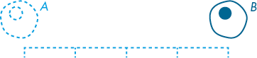
Figure 10-11: A magnitude of 4 units
A magnitude is a scalar value. It’s a single quantity you can describe by using a single value, like a floating-point number or integer. For instance, the numbers 4, 1.5, 42, and one million are all scalar.
A vector is described by multiple scalars. In other words, it can hold multiple floating-point or integer values. Figure 10-12 presents a vector labeled v as a line with an arrowhead at one end. The length of v is its magnitude; the slope and arrowhead indicate its specific direction.

Figure 10-12: The vector v extends 4 units right and 3 units up.
Each vector has an x and y component, so you can express this vector as v = (4, 3). It describes a force to move the amoeba to a new location 4 units to the right and 3 units up from its previous location. You denote vectors in boldface type, but it’s also common to draw a small arrow above the v in situations where bold is impractical (for example, for handwritten formulas).
The horizontal and vertical measurement lines in Figure 10-12 form a right triangle with v as its hypotenuse. From this triangle, you can calculate the magnitude of the vector by using the Pythagorean theorem. The theorem states that the square of the hypotenuse is equal to the sum of the squares of the other two sides.
If you add 4 squared (the adjacent side) to 3 squared (the opposite side), you get 25, the length of the hypotenuse squared. The square root of 25 is 5, the length of the hypotenuse and the magnitude of v. But you don’t need to worry about performing such calculations. Processing provides a built-in PVector class especially for working with vectors that includes, among other methods, a mag() for calculating magnitude.
You’ll adapt your amoeba sketch to work with the PVector class. While showing how to make your amoeba move with vectors, I’ll also outline how the various PVector methods work, revealing what’s happening on a mathematical level.
The PVector Class
PVector is a built-in Processing class for working with Euclidean vectors. You can use it anywhere in your sketch—no import line required. PVector can handle two- and three-dimensional vectors, but we’ll stick to the 2D variety here.
To create a new 2D vector, the PVector() class requires an x and y argument. For example, this line defines the vector depicted previously in Figure 10-12:
v = PVector(4, 3)The v instance is a new vector that extends 4 units across and 3 units up. You should, however, switch the 3 to -3 to match Processing’s coordinate system (where the y values decrease as you move up).
A vector can point in any direction, negative or positive, but the magnitude is always a positive value. Use the mag() method to calculate the magnitude of any PVector instance; for example:
magnitude = v.mag()
print(magnitude)  # displays 5.0
You know that the mag() method must invoke prewritten code based on the Pythagorean theorem. It returns a floating-point value of 5.0, confirming our calculations from the previous section.
Moving an Amoeba with PVector
You’ll create a PVector instance to animate amoeba a1 moving across the display window. In Chapter 6, you programmed something similar—a DVD screensaver—as you instructed Processing to move a DVD logo a set number of pixels horizontally and vertically in each frame for smooth, diagonal movements. The approach is similar here, but you’ll use the PVector class instead. You’ll find that the vector-based approach is more efficient for simulating movement and forces.
Switch to the amoeba.py tab and add a new propulsion vector to the __init__() method:
class Amoeba(object):

    def __init__(self, x, y, diameter, xspeed, yspeed):
        . . .
        self.propulsion = PVector(xspeed, yspeed)
The propulsion vector is initialized using two additional arguments for xspeed and yspeed that’ll determine how many pixels your amoeba is propelled horizontally and vertically in each frame. In comparison to the DVD screensaver task, here you’re combining the xspeed and yspeed variables into a single vector named propulsion.
Now switch to the microscopic tab. Use a fourth and fifth Amoeba() argument to set the x and y components of the propulsion vector to 3 and -1, respectively. Use the draw() function to increment your amoeba’s x and y attributes by those values:
. . .
a1 = Amoeba(400, 200, 100, 3, -1)
. . .
def draw():
    background('#004477')
    a1.x += a1.propulsion.x
    a1.y += a1.propulsion.y
    a1.display()
Each frame, amoeba a1’s x value increases by 3 pixels; at the same time, its y value decreases by 1. In the default Processing coordinate system, reducing y moves the amoeba up. If you run the sketch, the amoeba should move (quite rapidly) along a diagonal trajectory, starting in the center of the display window and soon exiting just below the upper right corner.
You can also use a PVector instance to store your amoeba’s x- and y-coordinates. In fact, you can use PVector to store any x-y coordinate pair; after all, it’s an object used to store two (or three) numbers, which also includes a bunch of handy methods for performing vector operations. Switch to the amoeba.py tab; replace the self.x and self.y attributes with a new vector named self.location:
class Amoeba(object):

    def __init__(self, x, y, diameter):
        print('amoeba initialized')
        self.location = PVector(x, y)
       . . .
The amoeba’s location is now a PVector instance too, albeit one that describes a point in the display window rather than a velocity or force. But you can’t rerun the sketch yet. First, you need to update the rest of the amoeba.py file to work with the new location attribute.
Your Amoeba class has multiple references to self.x and self.y, and you’ll need to ensure that you replace them all with self.location.x and self.location.y, respectively. The easiest way to do this is by using a find-and-replace operation. From the Processing menu bar, select Edit▶Find to access the Find tool (Figure 10-13). Enter self.x into the Find field, and self.location.x into the Replace with field. Click the Replace All button to apply the changes. The checkbox settings shouldn’t make any difference here. Once you’re done, do the same for self.y, replacing it with self.location.y.

Figure 10-13: The Processing Find (and Replace) tool
Now, change a1.x and a1.y in your microscopic tab to a1.location.x and a1.location.y, respectively:
    . . .
    a1.location.x += a1.propulsion.x
    a1.location.y += a1.propulsion.y
    . . .
You add the x components on one line and the y components on another. However, there’s a more efficient way to do this, using PVector addition.
Adding Vectors
The + operator is used to add floating-point numbers or integers. Additionally, it serves as a concatenation operator for string operands. The PVector class is programmed to work with the + operator too. You can add one PVector instance to another to get a vector that’s the sum of the two. By extension, += works as an augmented assignment operator, stating that the vector operand to the left of the operator is equal to itself plus the right operand.
Replace your a1.x += propulsion.x and a1.y += propulsion.y lines with a single line to add the propulsion and location, adding PVector instances rather than individual components:
. . .
def draw():
    background('#004477')
    a1.location += a1.propulsion
    a1.display()
With each call of the draw() function (every frame), the amoeba location is incremented by the propulsion vector. If you run the sketch, the amoeba moves along the same trajectory as before, 3 pixels across and 1 up each frame, exiting just below the upper right corner of the display window.
Let’s add a new force to the simulation. You’ll model a current flowing diagonally across the display window; it assists the amoeba’s prevailing motion, flowing toward northeast. As Wikipedia (https://en.wikipedia.org/wiki/Current_(fluid)) defines it, “A current in a fluid is the magnitude and direction of flow within that fluid.” Evidently, this is something to model using a vector.
Add a new PVector named current to your microscopic tab. Add that vector to your location each frame by using the draw() function:
. . .
current = PVector(1, -2)
. . .
def draw():
    background('#004477')
    a1.location += a1.propulsion
    a1.location += current
    a1.display()
The propulsion vector is angled at roughly 18 degrees, pushing more rightward than upward. The current vector is angled at approximately 63 degrees, pushing more upward than rightward (Figure 10-14). This combination makes the amoeba move faster, at an angle somewhere between the two vectors (~36 degrees). If you run the sketch, the amoeba should exit the top edge of the display window (before, it exited at the right edge).
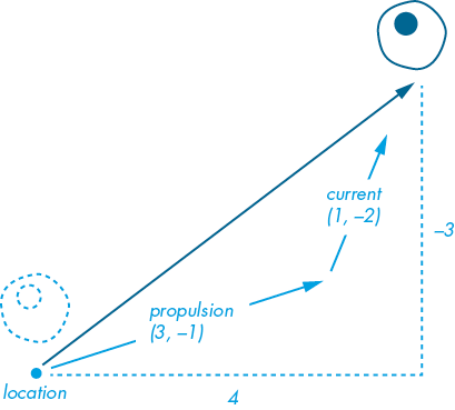
Figure 10-14: The amoeba moves a total of 4 pixels across and 3 up each frame.
Vector addition works by adding the x component of one vector to the x component of another, and likewise for the y components. In this case, adding the x components (3 + 1) equals 4, and adding the y components (–1 + –2) equals –3 . Regardless of the order in which you add vectors, the result is always the same. For example, (3, –1) + (1, –2) is the same as (1, –2) + (3, –1), and the resultant vector is (4, –3) in both instances. This makes vector addition a commutative operation, because changing the order of your operands doesn’t change the result.
You can experiment with different current values to see what happens. A current vector of (–3, 1) cancels out the propulsion vector exactly, and the amoeba won’t move from the center of the display window. A current vector of (–3.5, 1) will overpower the propulsion’s x component and exactly match the y component, moving the amoeba slowly and directly leftward.
The neat thing about this system is that you can add as many forces to the object’s location as you like. For instance, you might include a vector for wind, one for gravity, and so on.
Subtracting Vectors
In mathematics, the result of a subtraction operation is called the difference. For example, when you subtract 4 from 6, you’re left with a difference of 2. Likewise, when you subtract one vector from another, the resultant vector is the difference between the two.
You can picture vector subtraction like this: begin by placing the two vectors tail to tail; between the head of each vector, draw a line; this new line is the difference vector. In Figure 10-15, you subtract b from a; the difference (dark blue vector c) is (–2, –1).

Figure 10-15: Vector c is equal to (–2, –1).
The process of vector subtraction is similar to vector addition, but rather than adding the x (with x) and y (with y) components of each vector, you’re subtracting them. Note, however, that subtraction is noncommutative. That means, changing the order of the operands changes the result. For example, if you subtract a from b, you get (2, 1) instead of (–2, –1). This makes vector c point the opposite way, switching its head and tail.
You can subtract PVector instances by using the – operator. Here’s an example:
print(current - a1.propulsion)If your current vector is equal to (1, –2), this will print [-2.0, -1.0, 0.0] to the console. Processing prints a PVector instance as a list of three floating-point values, which represent the vector’s x, y, and z components, respectively. The z value is always a 0, unless you’re working with three-dimensional vectors.
You’ve added a propulsion and current vector to the amoeba’s location to get it moving across the display window. You’ll now apply what you’ve learned about vector subtraction to get the amoeba moving toward your mouse pointer. You’ll create a new PVector instance called pointer to store the x-y coordinates of your mouse pointer. You’ll subtract location (which holds the amoeba’s x-y coordinates) from pointer to find the difference vector (Figure 10-16), which you’ll use to redirect the amoeba.
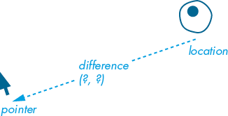
Figure 10-16: The difference vector is equal to pointer – location.
Ensure that your current vector is set to (1, –2). Add a new PVector named pointer and a difference variable that’s equal to the pointer minus the amoeba location (the difference vector depicted in Figure 10-16).
. . .
current = PVector(1, -2)
. . .
def draw():
    background('#004477')
    pointer = PVector(mouseX, mouseY)
    difference = pointer - a1.location
    a1.location += difference
    . . .
The mouseX and mouseY are Processing system variables that hold the x- and y-coordinates of your mouse pointer. Note, however, that Processing can begin tracking the mouse position only after you move the pointer in front of the display window; until that time, mouseX and mouseY both return a default value of 0.
If you run the sketch, the amoeba will attach to the mouse pointer. This happens because the amoeba reaches the pointer position in a single “leap.” Instead, you want the amoeba to “swim” toward the pointer, advancing in small increments over multiple frames.
Limiting Vector Magnitude
The PVector class provides the limit() method to limit the magnitude of any vector, which does not affect the direction. It requires a scalar (integer or floating-point) argument that represents a maximum magnitude.
You’ll use the difference vector to steer the amoeba toward the mouse pointer by adding it to the propulsion vector. You’ll limit the propulsion vector to a magnitude of 3 (Figure 10-17), enough to overpower the current marginally (which has a magnitude of 2.24) when the amoeba is swimming directly into it.

Figure 10-17: The propulsion vector’s magnitude is limited to 3.
Make the following insertions/changes to the draw() function to steer and propel the amoeba toward the mouse pointer:
. . .
def draw():
    . . .
 1 #a1.location += difference
 2 a1.propulsion += difference.limit(0.03)
 3 a1.location += a1.propulsion.limit(3)
    a1.location += current
    a1.display()
First, comment out or delete the existing a1.location += difference line 1. The limit() method restricts the difference vector to a magnitude of 0.03 2. This tiny value is added to the propulsion vector each frame—the effect rapidly accumulating—steering the amoeba progressively toward the mouse pointer. But even when the amoeba is heading directly at the pointer, the propulsion vector’s magnitude will not exceed 3 3.
Run the sketch and position your mouse pointer over the display window somewhere near the lower left corner. The amoeba will have drifted out of view. But wait for a while, and it’ll slowly make its way toward the corner; when it reaches the pointer, it will overshoot it slightly, then turn around and overshoot it on the way back. It continues to overshoot the pointer, because it’s trying to reach its target as quickly as possible. Now move your pointer to the lower right corner. Assisted by the current, the amoeba is quick to reach the opposite side of the screen, but its higher velocity leads it to overshoot the target dramatically.
Soon, you’ll add multiple amoebas to the simulation. To prepare them for moving at different speeds, add an attribute for maximum propulsion to the Amoeba class:
class Amoeba(object):

    def __init__(self, x, y, diameter, xspeed, yspeed):
        . . .
        self.maxpropulsion = self.propulsion.mag()
This attribute will limit the magnitude/power of the amoeba’s propulsion vector based on the xspeed and yspeed arguments you provide. Adapt the code in your microscopic tab to work with the maxpropulsion attribute, switching out the arguments of both limit() methods. Additionally, adjust the values for the xspeed, yspeed, and the current vector, reducing them by a factor of 10:
. . .
a1 = Amoeba(400, 200, 100, 0.3, -0.1)
current = PVector(0.1, -0.2)
. . .
def draw():
    . . .
    a1.propulsion += difference.limit(a1.maxpropulsion/100)
    a1.location += a1.propulsion.limit(a1.maxpropulsion)
    . . .
The reduced propulsion and current values slow down the simulation, so the amoeba movement is more steady and controlled. The amoeba won’t wildly overshoot its target anymore, but it still makes small orbits around the pointer. The limit for the difference vector is now proportional to the amoeba’s maximum propulsion, so a faster amoeba has some extra steering power to handle its higher velocity.
Performing Other Vector Operations
There’s more to vectors and the PVector class, but that’s all I cover in this book. Consider what you’ve learned as an elementary introduction to the topic. The PVector class can additionally handle vector multiplication, division, normalization, 3D vectors, and more. Vectors are useful for programming anything that requires physics, like video games, and you’re likely to reencounter them in your creative coding adventures.
Adding Many Amoebas to the Simulation
You have a working amoeba module, but you’re still dealing with a single amoeba instance, a1, so the next step is to create a colony. You can create as many instances as you like from a single class. In this section, you’ll spawn eight amoebas in the same display window by using the Amoeba class. Each amoeba will vary in size, and you’ll start them at different x-y coordinates. Recall that each amoeba instance includes a dictionary of randomized nucleus values, so the nuclei will vary too.
One (rather manual) approach for adding amoebas is to define additional instances with personalized variable names, with explicitly differentiated parameters. Consider these three new amoeba:
a1 = Amoeba(400, 200, 100, 0.3, -0.1)
sam = Amoeba(643, 105, 56, 0.4, -0.4)
bob = Amoeba(295, 341, 108, -0.3, -0.1)
lee = Amoeba(97, 182, 198, -0.1, 0.2)
. . .
You can keep adding amoebas in this manner, but the approach has its downsides. For one, you need to remember to call every display() method in the body of the draw() function to render each amoeba:
def draw():
    . . .
    a1.display()
    sam.display()
    bob.display()
    lee.display()
    . . .
This will display sam, bob, and lee standing still; to get those amoebas moving, the draw() function requires even more code. That isn’t especially efficient if you’re dealing with 5 or so amoebas, never mind 100.
Personalized amoeba names are cute and all, but not important for this program. Instead, you’ll store the amoebas in a list. You can conveniently use a loop to generate a list of as many amoebas as you like. Then you can call each amoeba’s display() method (along with the code to move it) by using another loop.
Replace the a1 line at the top of your microscopic code with an empty amoebas list and a loop to populate it:
from amoeba import Amoeba

amoebas = []

for i in range(8):
    diameter = random(50, 200)
    speed = 1000 / (diameter * 50)
    x, y = random(800), random(400)
    amoebas.append(Amoeba(x, y, diameter, speed, speed))
. . .
With each iteration of the for loop, Python creates a new Amoeba() instance. The Amoeba() arguments are randomized to vary the x-coordinate, y-coordinate, and diameter of each instance. The speed value is based on the diameter—so bigger amoebas move slower (recall that the propulsion and maxpropulsion attribute is derived from the xspeed and yspeed arguments). The append() method adds the new amoeba instance to the amoebas list. The amoebas don’t have names like sam, bob, and lee, but you can address them by index as amoebas[0], amoebas[1], and so forth.
You must add a for loop to the draw() function to render the full list of amoebas. Here’s your amended code:
. . .
def draw():
    background('#004477')
    pointer = PVector(mouseX, mouseY)

    for a in amoebas:
        difference = pointer - a.location
        a.propulsion += difference.limit(a.maxpropulsion/100)
        a.location += a.propulsion.limit(a.maxpropulsion)
        a.location += current
        a.display()
The for loop iterates the entire amoebas list. For each amoeba, it calculates an updated location, and then renders that amoeba by using its display() method.
The larger, slower amoebas might drift out of the display window, overwhelmed by the current, never to be seen again. To avoid this problem, add code for wraparound edges—so that if an amoeba exits the display window, it reappears on the opposite side, maintaining its speed and trajectory:
    . . .
    for a in amoebas:
        . . .
        r = a.d / 2

        if a.location.x - r > width:
            a.location.x = 0 - r
        if a.location.x + r < 0:
            a.location.x = width + r
        if a.location.y - r > height:
            a.location.y = 0 - r
        if a.location.y + r < 0:
            a.location.y = height + r
The four if statements check each edge of the display window. It’s necessary to incorporate the radius (variable r) in the conditions to ensure that the amoeba has fully left the display window before it reappears on the opposite side. Likewise, each corresponding destination is offset by r to prevent the amoeba from reappearing halfway over the opposite edge. You can set r to 0 if you’d like to see what happens otherwise.
Each time you run the sketch, you get a different selection of amoebas. They all swarm toward your mouse pointer (although the current overpowers some of the large, slow ones), overlapping one another in the process. Figure 10-18 shows an example with eight amoebas.
To add or remove amoebas, you can adjust the argument in the range() function of your first loop, and the loop in the draw() function will adapt dynamically. If your computer seems to be struggling, you can reduce the number of amoebas.
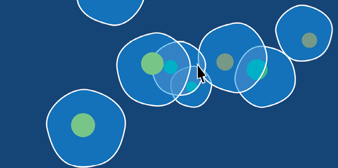
Figure 10-18: A display window with eight amoebas moving toward the mouse pointer
Challenge #10: Collision Detection
The amoebas can overlap one another. To prevent this from happening, you must first detect where overlaps occur. From there, you can apply vector forces to push any colliding pairs apart.
The amoebas are roughly circular, so a circle-circle collision detection algorithm will work nicely here. To understand how circle-circle collision detection works, refer to Figure 10-19. The pair of circles on the left have not collided; on the right is a colliding pair. For the non-colliding circles, the distance between the centers of each circle is greater than the sum of the two radii (r1 and r2). Conversely, where the circles have collided, the distance is less than the sum of the two radii.
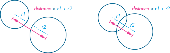
Figure 10-19: Circle-circle collision detection
To test for collisions in Processing, you’ll need to check each amoeba against every other amoeba in the amoebas list. For this purpose, add another for loop within the a in amoebas loop:
    . . .
    for a in amoebas:
        . . .
        for b in amoebas:

            if a is b:
                continue

            # your solution goes here
You don’t want to check whether an amoeba is colliding with itself. At the top of the loop, there’s an if a is b test. The is operator compares the objects on either side of itself to determine whether they point to the same instance; if a is the same instance as b, this will evaluate as True. The continue line terminates the current iteration of the loop to start at the beginning of the next, so your “solution” code is skipped.
Think about how you can use the distance vectors shown in Figure 10-19 to push apart colliding amoebas. Can you add (or subtract) a fraction of the distance vector to push an amoeba in the opposite direction to the one it has collided with?
If you need help, you can access the solution at https://github.com/tabreturn/processing.py-book/tree/master/chapter-10-object-oriented_programming_and_pvector/.
Summary
In this chapter, you learned how to use object-oriented programming to model real-world objects in Python. You defined a new Amoeba class, to which you added attributes and methods. A class serves as an object template, from which you can create countless instances. Grouping related variables (attributes) and functions (methods) into classes can help you structure code more efficiently. This is especially effective for programming larger, more complex projects.
You also learned how to separate classes (and other code) into different Python files, called modules, and how to use those modules to share code between projects or as reusable components among files in the same project. Remember that modules reduce the line count of the main sketch, allowing you to focus on higher-level logic.
This chapter also introduced Processing’s built-in PVector class for dealing with Euclidean vectors. A Euclidean vector describes a quantity that has both magnitude and direction, but you can also use a vector to store something’s location (as an x-y coordinate). In this chapter, you used vectors to simulate forces and control the positions of various objects in the display window.
In the next chapter, you’ll learn how to handle mouse and keyboard interaction in Processing. I’ve already touched on the mouseX and mouseY system variables in this chapter. However, you can do much more with capturing mouse clicks and keypresses, unlocking exciting ways to interact with your Processing sketches.