Chapter 11: Mitigating Quantum Errors Using Ignis

Ignis, as described in the Qiskit library, is a framework that contains various functionalities, such as characterization, verification, and mitigation. What this means is that it provides the ability to characterize the effects of noise on the system, verify the performance capabilities of the various gates and circuits, and calibrate circuits to generate routines that lessen the errors in your results.

This chapter will cover these topics by taking you through the process of characterizing and estimating the decoherence of the qubits from noise models. This will help you visualize and mitigate errors after measuring your results. We'll also work on mitigating quantum errors from the results we get back from the quantum devices using some of the features from the Ignis library.

In quantum systems, this noise originates from various sources: thermal heat from electronics, decoherence, dephasing, connectivity, or signal loss. Here, we will see how to measure the effects of noise on a qubit, and how to mitigate readout error noise to optimize our results. In the end, we will compare and contrast the differences to better understand the effects and ways to mitigate them.

The following topics will be covered in this chapter:

• Generating the noise effects of relaxation
• Estimating T1 decoherence time
• Generating the noise effects of dephasing
• Estimating T2 decoherence time
• Estimating T2* (T2 star) decoherence time
• Visualizing the T1, T2, and T2* characterization
• Mitigating readout errors using measurement calibrations

In this chapter, we will cover one of the challenges faced by most systems: noise. By the end of the chapter, you will know how to generate test circuits used to estimate the characteristics of each qubit, measure varying noise effects, such as relaxation and dephasing, and visualize the characteristics of each qubit. Finally, you'll learn how to apply error mitigation techniques to help minimize the effects of noise, based on the measurement characteristics analyzed by the test circuit results.

Technical requirements

In this chapter, it is expected that you have some understanding of the effects of noise on electronic systems and how to simulate them on a quantum computer. This chapter will cover some refreshers on simulating noise; however, the recommendation for you is to review Chapter 10, Executing Circuits Using Qiskit Aer, to get an understanding of how to simulate noise on a simulator from the configuration information of a quantum computer. This will help you understand an end-to-end scenario to simulate and mitigate errors on a simulator based on a quantum computer. The results of the simulation will provide information that will be leveraged to mitigate your circuit results after executing your circuit on a quantum computer.

Here is the source code we'll be using throughout this book: https://github.com/PacktPublishing/Learn-Quantum-Computing-with-Python-and-IBM-Quantum-Experience. Here is the link for the CiA videos: https://bit.ly/35o5M80

Generating noise effects of relaxation

We learned in Chapter 10, Executing Circuits Using Qiskit Aer, that we can generate various noise models that are based on the configuration of a specified quantum computer. After the configuration information is extracted, we can then apply any one of an array of error functions to a simulator, which will reproduce similar error effects to what we would get from a quantum computer.

In this section, we will expand on that to learn how to execute test circuits and visualize the results from those tests. This will help us to understand how various noise models affect the results over time. The two effects we will review here are the two most common issues found in near-term quantum systems: relaxation and dephasing. These are critical errors as they can affect the quantum state information, which would result in erroneous responses.

Later on in this chapter, we will also look at readout errors, which is another common source that originates when the system is applying a measurement pulse, while in parallel, listening in on the acquisition channel. The results and conversion from analog to digital can introduce many errors as well.

Generating noise models and test circuits

We will start by testing one of the most common and important effects of noise in quantum systems: decoherence. The three main types of decoherence are T1, T2, and T2*. Each of these represents a type of decoherence effect on the qubit. In order to analyze the effects of relaxation (T1) and dephasing (T2/T2*), we will first need to create the test circuits for each of the three. These test circuits will help us run experiments to analyze the characterization of the device. We will begin by looking at each one of these individually so as to understand the differences between them and how to mitigate them when they are run on a real quantum device.

In order to properly analyze the decoherence effects, we will need to run various circuits with a specific number and types of gates. Lucky for us, Qiskit Ignis includes a method to generate these test circuits for us. For decoherence testing, we will use t1_circuits, t2_circuits, and t2star_circuits, which will generate the T1, T2, and T2* circuits, respectively. Let's take a quick moment to review what the decoherence of each one means as we create the test circuits.

Generating and executing T1 test circuits

T1, as we covered in Chapter 10, Executing Circuits Using Qiskit Aer, is often referred to as the relaxation time. Relaxation time refers to the time it takes the energy of a qubit to decay from the excited state (|1) back down to its ground state (|0) as illustrated in the following graph, where P(1) indicates the probability of 1, and P(0) is the probability of 0. The T1 time is defined as the value when P(t) = 1/e (refer to the following diagram):

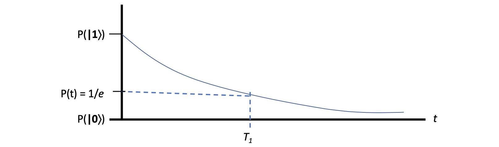
Figure 11.1 – T1 defined as the decay time where the probability of the energy state reaches 1/e

In order to determine the amount of time to reach T1 for any qubit, we will need to create a test circuit that places the qubit in an excited state, |1. This we know how to do by simply applying an X gate to the qubit.

Next, we will need to wait a certain amount of time before measuring the qubit. One way to do this is to insert an identity gate with a fixed gate time. This is a simple circuit to create manually; however, the challenge is to determine how many identity gates you need to include and how scalable that process is. Lucky for us, we have the t1_circuits method!

This method allows us to define how many gates to include in each circuit and the gate time for each identity gate, as well as list which qubits to apply to these gates. In the following code sample, we will generate an array of quantum circuits, each with an X gate and the number of identity gates we specified. We will also provide the gate times for the identity gates. Let's create a new IQX Qiskit notebook and insert the following code, which will load in additional helper math, plot, Aer, and Ignis libraries:

# Import plot and math libraries

import numpy as np

import matplotlib.pyplot as plt

# Import the noise models and some standard error methods

from qiskit.providers.aer.noise import NoiseModel

from qiskit.providers.aer.noise.errors.standard_errors import amplitude_damping_error, phase_damping_error

# Import all three coherence circuits generators and fitters

from qiskit.ignis.characterization.coherence import t1_circuits, t2_circuits, t2star_circuits

from qiskit.ignis.characterization.coherence import T1Fitter, T2Fitter, T2StarFitter

Now that we have our Ignis libraries loaded, we can use them to generate the test circuits, as illustrated in the following cell. We will generate a list of the number of identity gates to include in each test circuit and include the gate time for each identity gate. The qubit we will measure for T1 will be the first qubit.

We will use the same name of the parameters listed in the t1_circuits API documentation – num_of_gates, gate_time, and qubits – where the array length of the number of gates relates to the number of test circuits we will create, which in this case is 18, where out of which 12 are linearly spaced and 6 are manually defined entries. In the following code, we will define the variables to generate an array of test circuits:

# Generate the T1 test circuits

# Generate a list of number of gates to add to each circuit

# using np.linspace so that the number of gates increases # linearly

# and append with a large span at the end of the list (200-# 4000)

num_of_gates = np.append((np.linspace(1, 100, 12)).astype(int), np.array([200, 400, 800, 1000, 2000, 4000]))

#Define the gate time for each Identity gate

gate_time = 0.1

# Select the first qubit as the one we wish to measure T1

qubits = [0]

# Generate the test circuits given the above parameters

test_circuits, delay_times = t1_circuits(num_of_gates, gate_time, qubits)

# The number of I gates appended for each circuit

print('Number of gates per test circuit: ', num_of_gates, ' ')

# The gate time of each circuit (number of I gates * gate_time)

print('Delay times for each test circuit created, respectively: ', delay_times)

After generating an array of test circuits and their respective delay times, this will print out the number of gates that will be appended to each test circuit and the delay times for each circuit, respectively, as follows:

Number of gates per test circuit:

[   1   10   19   28   37   46   55   64   73   82   91  100   200  400 800 1000 2000 4000]

Delay times for each test circuit created, respectively:

[1.0e-01 1.0e+00 1.9e+00 2.8e+00 3.7e+00 4.6e+00 5.5e+00 6.4e+00 7.3e+00 8.2e+00 9.1e+00 1.0e+01 2.0e+01 4.0e+01 8.0e+01 1.0e+02 2.0e+02 4.0e+02]

Let's confirm a few things about the test circuits we created. We know that in total, the number of test circuits created should be 18. Then, we will draw the first circuit, which should include the X gate to set the qubit in the excited state, followed by one identity gate before the measurement:

print('Total test circuits created: ', len(test_circuits))

print('Test circuit 1 with 1 Identity gate:')

test_circuits[0].draw()

The results confirm our expectation of 18 test circuits and a single identity gate:

Total test circuits created: 18

The following circuit diagram shows test circuit 1 with one identity gate:

Figure 11.2 – Test circuit 1, with an X gate and a single identity gate

With the gate time of the identity gate set to 0.1, we know that this is a fairly quick result. Let's look at the next test circuit to see how it increases:

print('Test circuit 2 with 10 Identity gates:')

test_circuits[1].draw()

In the second test circuit, we see that we now have 10 identity gates, which increases our delay time from 0.1 in the first circuit to 1.0 in the second circuit. The following circuit diagram shows you test circuit 2 with 10 identity gates:

Figure 11.3 – Test circuit 2, with an X gate and 10 identity gates

Next, we will generate a simulator with an amplitude damping error applied to the identity gate on qubit 0:

# Set the simulator with amplitude damping noise

# Set the amplitude damping noise channel parameters T1 and # Lambda

t1 = 20

lam = np.exp(-gate_time/t1)

# Generate the amplitude dampling error channel

error = amplitude_damping_error(1 - lam)

noise_model = NoiseModel()

# Set the dampling error to the ID gate on qubit 0.

noise_model.add_quantum_error(error, 'id', [0])

Next, we will execute all our test circuits on the simulator with the generated noise model:

# Run the simulator with the generated noise model

backend = Aer.get_backend('qasm_simulator')

shots = 200

backend_result = execute(test_circuits, backend, shots=shots, noise_model=noise_model).result()

Let's review our results. The first test circuit, which comprised only one identity gate, should, along with the noise model effects, display a very small error in our results:

# Plot the noisy results of the largest (last in the list) # circuit

plot_histogram(backend_result.get_counts(test_circuits[0]))

As expected, we observe a very small, almost insignificant result of the amplitude decay down to the ground state:

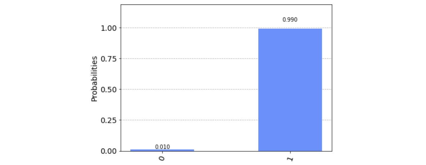
Figure 11.4 – The results from the first test circuit, with an insignificant error rate

Now, let's take a look at the other side and view the results from the last test circuit. Here, we have a total of 4,000 gates; the results, as we will see, are quite significant:

# Plot the noisy results of the largest (last in the list) # circuit

plot_histogram(backend_result.get_counts(test_    circuits[len(test_circuits)-1]))

As you can see in the histogram, the results are entirely back to the ground state, indicating that we have surpassed the T1 time and that the execution of our last test circuit has resulted in every count being reverted back down to the ground state:

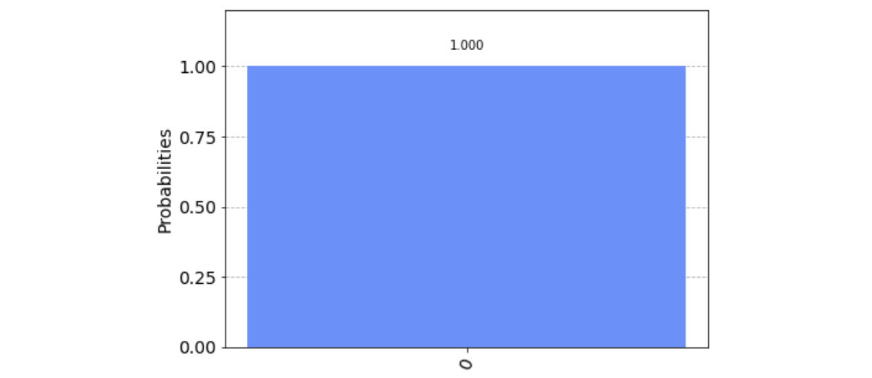
Figure 11.5 – Results from test circuit 18 with 4,000 identity gates, with significant errors

Now that we have created and executed our test circuits for T1, we can analyze and use fitters to estimate the T1 time based on the results of our test circuits.

Estimating T1 decoherence times

Fitters are used to estimate the T1 time based on experiment results from t1_circuits executed on noisy devices. The estimate is based on the probability formula of measuring 1 from the following equation, where A, T1, and B are unknown parameters:

Since we set the T1 value earlier when we defined the noise model of the qubit as 20, let's assume for now that we do not know that and initialize the value to some percentage value away from the actual value. The T1Fitter class has a few parameters that it needs in order to characterize the qubit. We will start by initializing the values for a, t1, and b:

# Initialize the parameters for the T1Fitter, A, T1, and B

param_t1 = t1*1.2

param_a = 1.0

param_b = 0.0

This will initialize our t1, a, and b parameters, which we will use to generate T1Fitter.

Next, we will generate T1Fitter by providing the following parameters:

• backend_result: The results from our test circuits on the backend
• Xdata: The delay times for the test circuits
• qubits: The qubits that we wish to use to measure T1
• fit_p0: The initial values to set A, T1, and B, respectively (these must be entered in order)
• fit_bounds: The tuple representing the lower and upper bounds for the parameters to fit
• time_unit: The unit of the delay time in xdata

Referencing the parameters from the test circuits, we can generate and plot the results of T1Fitter, as follows:

# Generate the T1Fitter for our test circuit results

fit = T1Fitter(backend_result, delay_times, qubits,

               fit_p0=[param_a, param_t1, param_b],

               fit_bounds=([0, 0, -1], [2, param_t1*2, 1]))

# Plot the fitter results for T1 over each test circuit's delay # time

fit.plot(0)

The result will plot the relaxation decay of the qubit over the delay times of each test circuit. You can see the decay results as follows:

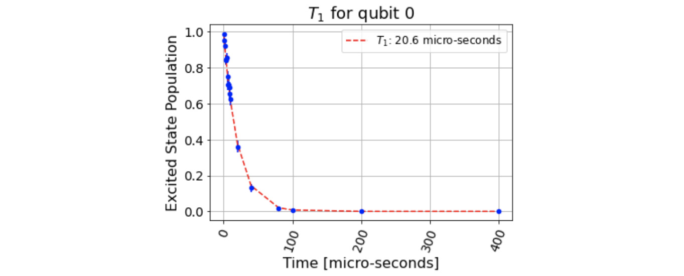
Figure 11.6 – T1Fitter estimated results, where T1 is estimated to be at 20.6 microseconds for qubit 0

In this section, you have generated T1 test circuits, executed them with amplitude dampening noise models on a backend device, and characterized the results to estimate T1. Characterizing other qubits can be done as well by simply listing the other qubit indices; in this example, we chose to characterize qubit [0]. Let's now characterize T2 and T2* on a qubit. The steps you will see are very similar.

Generating the noise effects of dephasing

T2 and T2* are similar in that they are both representing the dephasing of a qubit. The difference is in the experimental process they conduct to measure each circuit. Determining the decay time of T2* is conducted by placing the qubit in a superposition state using a Hadamard gate, then after some delay time, you apply another Hadamard gate and measure. This should result in the qubit returning to the originating state – in this case, the grounded state. This experiment is referred to as the Ramsey experiment.

To determine the decay time of T2, we will perform a similar experiment as we did for T2*, by first placing the qubit in a superposition state. The difference is that rather than waiting for some delay time before applying another Hadamard gate before measuring, you instead wait until half the delay time and then apply either an X or Y rotation, then wait until the second half delay time is complete before taking the measurement. This experiment is referred to as the Hahn echo experiment.

In all, both experiments will measure the decay time of the dephasing where the expectation of the result is random. In the next section, we will generate the T2 circuits based on the Ramsey experiment.

Generating and executing T2 circuits

T2 is often referred to as the dephasing time. Rather than looking at the relaxation of a qubit from the excited state to the ground state, the dephasing of a qubit has more to do when the state is in a linear combination of the two states. Let's step through what is meant here by dephasing:

1. When a qubit transitions from the ground state, |0, to the superposition state, |+, after we run a Hadamard gate on the qubit, we expect that by adding another Hadamard gate, the qubit will then return to the ground state, |0.
2. However, while the qubit is in the |+ state, this is where dephasing could be a problem. The problem lies in that over time, the qubit may or may not be in the |+ or state, but rather in some angle around the Z axis away from the |+ state.
3. This would then render the qubit unpredictable when applying another Hadamard gate if our expectation is for the qubit to return to the ground state but instead is found in the excited state, |1.

In order to test this, we will need a test circuit that will first place the qubit from the initial state, |0, into the superposition state, |+. This, as we know, can be done with a Hadamard gate. Then, we can place an identity gate to increase the delay time between each step. Just as before, we will import a few libraries and define the parameters for the t2_circuits generator method by entering the following:

# Import the thermal relaxation error we will use to create our # error

from qiskit.providers.aer.noise.errors.standard_errors import thermal_relaxation_error

# Import the T2Fitter Class and t2_circuits method

from qiskit.ignis.characterization.coherence import T2Fitter

from qiskit.ignis.characterization.coherence import t2_circuits

Now that we have the necessary classes and method, we'll define our t2_circuits parameters in the next cell:

num_of_gates = (np.linspace(1, 300, 50)).astype(int)

gate_time = 0.1

# Note that it is possible to measure several qubits in # parallel

qubits = [0]

t2echo_test_circuits, t2echo_delay_times = t2_circuits(num_of_gates, gate_time, qubits)

# The number of I gates appended for each circuit

print('Number of gates per test circuit: ', num_of_gates, ' ')

# The gate time of each circuit (number of I gates * gate_time)

print('Delay times for T2 echo test circuits: ', t2echo_delay_times)

Running the preceding cell results in the following number of gates and delay times to generate our T2 test circuits:

Number of gates per test circuit:

[  1   7  13  19  25  31  37  43  49  55  62  68  74  80  86   92  98 104 110 116 123 129 135 141 147 153 159 165 171 177 184

190 196 202 208 214 220 226 232 238 245 251 257 263 269 275 281 287 293 300]

Delay times for T2 echo test circuits:

[ 0.2  1.4  2.6  3.8  5.   6.2  7.4  8.6  9.8 11.  12.4 13.6 14.8 16.

17.2 18.4 19.6 20.8 22.  23.2 24.6 25.8 27.  28.2 29.4 30.6 31.8 33.

34.2 35.4 36.8 38.  39.2 40.4 41.6 42.8 44.  45.2 46.4 47.6 49.  50.2

51.4 52.6 53.8 55.  56.2 57.4 58.6 60. ]

As in the previous test circuit example, let's examine the first test circuit to confirm that the gates are where we expect to see them:

# Draw the first T2 test circuit

t2echo_test_circuits[0].draw()

This naturally results in the following test circuit. Note that the Y rotation gate is located in the middle:

Figure 11.7 – T2 test circuit with Hadamard rotations on each end and a Y rotation in the middle of the identity gates

This is the Ramsey experiment test circuit we will be running. The other 49 test circuits we generated are increasing in size and will eventually surpass the T2 time, which produces random results.

Let's now generate our T2 noise model to include in the simulator. This will allow us to include only a thermal_relaxation_error model in the circuit, so when we execute our circuit, this is the only noise effect. We will then store our noise results in the t2_echo_backend_result variable:

# We'll create a noise model on the backend simulator

backend = Aer.get_backend('qasm_simulator')

shots = 400

# set the t2 decay time

t2 = 25.0

# Define the T2 noise model based on the thermal relaxation # error model

t2_noise_model = NoiseModel()

t2_noise_model.add_quantum_error(thermal_relaxation_error(np.inf, t2, gate_time, 0.5), 'id', [0])

# Execute the circuit on the noisy backend

t2echo_backend_result = execute(t2echo_test_circuits, backend,                         shots=shots,

                        noise_model=t2_noise_model,                         optimization_level=0).result()

Next, let's plot our results, starting with the first test circuit with the shortest delay time, and then the last test circuit with most delay time:

plot_histogram(t2echo_backend_result.get_counts(t2echo_test_    circuits[0]))

This results in an expected ground state, which is denoted as follows, where we have a 99% probability of measuring 0 (very minimal effects of dephasing time):

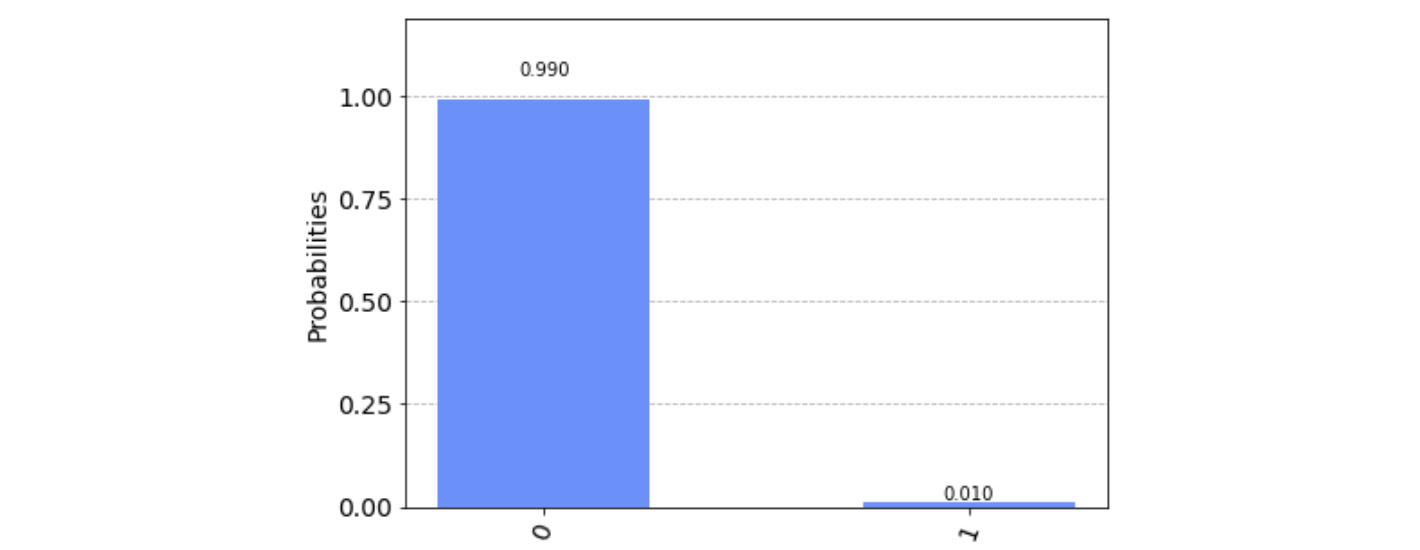
Figure 11.8 – The first T2 test circuit executed on the noisy backend

Now, let's see the last test circuit's results:

plot_histogram(t2echo_backend_result.get_counts(t2echo_test_    circuits[len(t2echo_test_circuits)-1]))

This, as we can see, has a fairly equal probability of either of the two basis states, which indicates that we have far exceeded the dephasing time, T2 (exceeds the T2 dephasing time):

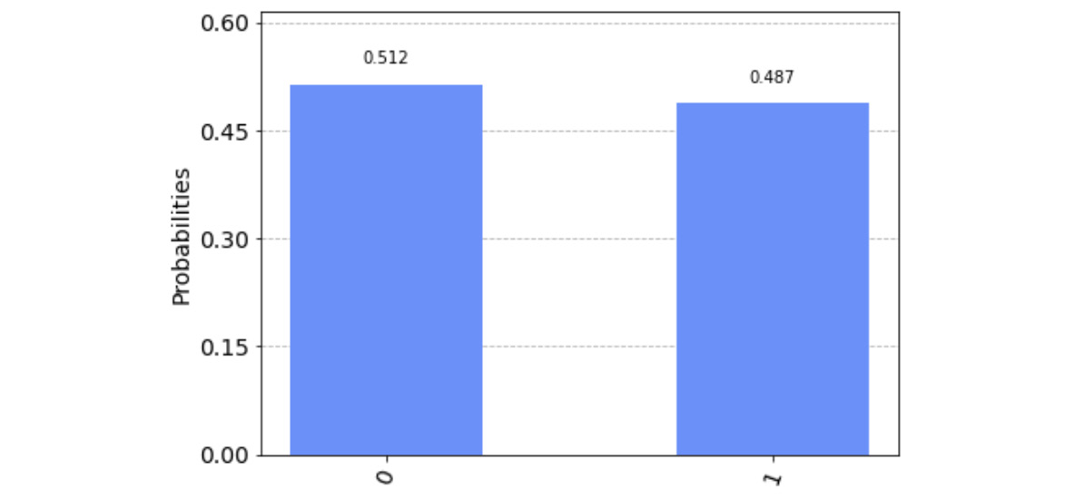
Figure 11.9 – The last T2 test circuit executed on the noisy backend

What we saw here is how, over time, we can see that the dephasing time greatly affects our results. This dephasing time gets very problematic if not mitigated. Mitigating errors will be described later in this section, Mitigating readout errors.

Estimating T2 decoherence times

We estimate the T2 time based on experiment results from t2_circuits executed on noisy devices. The estimate is based on the probability formula of measuring 0 from the following equation, where A, T2, and B are unknown parameters:

Finally, to estimate T2* and characterize the qubit with respect to the results, we will leverage T2Fitter. To generate the T2Fitter class, we will use similar parameter definitions as T1Fitter in the previous section, only this time, we will use the results from the T2 test circuits:

# Generate the T2Fitter class using similar parameters as the # T1Fitter

t2echo_fit = T2Fitter(t2echo_backend_result, t2echo_delay_times, qubits, fit_p0=[0.5, t2, 0.5], fit_bounds=([-0.5, 0, -0.5], [1.5, 40, 1.5]))

# Print and plot the results

print(t2echo_fit.params)

t2echo_fit.plot(0)

plt.show()

The preceding code prints out the estimate values for A, T2, and B for qubit 0:

{'0': [array([ 0.52397653, 27.06685838, 0.47677457])]}

The previous code also plots the characterization of qubit 0, with an estimated value for T2 at 27.1 ms:

Figure 11.10 – Plot T2Fitter characterization of qubit 0, where T2 is estimated to be at 27.1 ms

Now, that we have completed characterizing T2 on qubit 0, let's look at the last characterization example of T2*.

Generating and executing T2* test circuits

T2* is also referred to as the dephasing time of a qubit. As mentioned earlier, the difference is in the experiment, where in the previous experiment for T2, we added an array of identity gates before rotating the state of the qubit with a Y gate.

For T2*, we will generate test circuits that place the qubit in a superposition state and then after some delay time, it will apply a linear phase gate, immediately followed by a reversing the superposition back to the initial state. The test circuit will also include the induced oscillation frequency on the phase gate. We'll create the test circuits using the t2star_circuits method by creating it as described in the following cell:

# 50 total linearly spaced number of gates

# 30 from 10->150, 20 from 160->450

num_of_gates = np.append((np.linspace(1, 150, 30)).astype(int), (np.linspace(160,450,20)).astype(int))

# Set the Identity gate delay time

gate_time = 0.1

# Select the qubit to measure T2*

qubits = [0]

# Generate the 50 test circuits with number of oscillations set # to 4

test_circuits, delay_times, osc_freq = t2star_circuits(num_of_gates, gate_time, qubits, nosc=4)

print('Circuits generated: ', len(test_circuits))

print('Delay times: ', delay_times)

print('Oscillating frequency: ', osc_freq)

This will produce the 50 test circuits, with the specified delay time for each identity gate and the oscillating frequency for the phase gate:

Circuits generated:  50

Delay times:  [ 0.1  0.6  1.1  1.6  2.1  2.6  3.1  3.6  4.2  4.7  5.2  5.7  6.2  6.7

7.2  7.8  8.3  8.8  9.3  9.8 10.3 10.8 11.4 11.9 12.4 12.9 13.4 13.9

14.4 15.  16.  17.5 19.  20.5 22.1 23.6 25.1 26.6 28.2 29.7 31.2 32.7

34.3 35.8 37.3 38.8 40.4 41.9 43.4 45. ]

Oscillating frequency:  0.08888888888888889

Let's confirm the first test circuit and see how many identity gates are generated:

print(test_circuits[0].count_ops())

test_circuits[0].draw()

As we can see, this generates one identity gate, followed by a phase gate, surrounded by Hadamard gates:

Figure 11.11 – The first test circuit, comprising an H, I, Phase, and then another H gate

If we look at the second test circuit, we should expect to see six identity gates followed by a phase gate, also surrounded by Hadamard gates:

print(test_circuits[1].count_ops())

test_circuits[1].draw()

We can now confirm that the T2* test circuits have been generated according to our parameters:

OrderedDict([('barrier', 8), ('id', 6), ('h', 2), ('u1', 1), ('measure', 1)])

We can also confirm that we have the six expected identity gates, followed by a phase gate, all of which are surrounded by Hadamard gates:

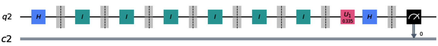
Figure 11.12 – The second test circuit, comprising an H, 6 Is, a Phase, and an H gate

These test circuits implement the Hahn echo experiment. Let's now execute these test circuits on a noisy backend; this time we will use a phase damping error to generate our noise model:

# Get the backend to execute the test circuits

backend = Aer.get_backend('qasm_simulator')

# Set the T2* value to 10

t2Star = 10

# Set the phase damping error and add it to the noise model to # the Identity gates

error = phase_damping_error(1 - np.exp(-2*gate_time/t2Star))

noise_model = NoiseModel()

noise_model.add_quantum_error(error, 'id', [0])

# Run the simulator

shots = 1024

backend_result = execute(test_circuits, backend, shots=shots, noise_model=noise_model).result()

Let's view the first test circuit, which should have minimal effects of T2*:

# Plot the noisy results of the shortest (first in the list) # circuit

plot_histogram(backend_result.get_counts(test_circuits[0]))

As expected, this illustrates very minimal effects of T2*. As you can see, we have a 99% probability of measuring 0, which is the expected result from this test circuit:

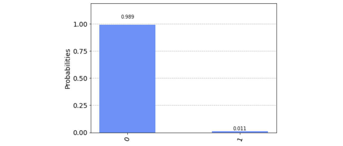
Figure 11.13 – Results of the first test circuit, with minimal T2* effects

We will review the results from the last test circuit. Due to the fact that this has the longest delay time, we should see the maximum effect of T2*:

# Plot the noisy results of the largest (last in the list) # circuit

plot_histogram(backend_result.get_counts(test_circuits[len(test_circuits)-1]))

As expected, the results are now completely random:

Figure 11.14 – Results of the last test circuit, with maximum T2* effects

We've successfully completed generating the T2* test circuits and obtained their results from executing them on a noisy backend. Next, we will estimate the T2* dephasing time and characterize the effects on qubit 0.

Estimating the T2* dephasing time

We will estimate the T2* dephasing time based on the experiment results from t2star_circuits executed on a noisy device. We will use the probability formula of measuring 0 from the following equation, where A, T2*, f, , and B are unknown parameters:

The T2StarFitter parameters are the same, with the exception of the following:

• fit_p0: The initial values to the fit parameters – in order, A, T2*, f, , B.
• fit_bounds: The lower and upper bounds, respectively. Parameters in order: A, T2*, f, , B

The following code will set the initial parameter values so that we can generate our T2StarFitter and bounds:

# Set the initial values of the T2StarFitter parameters

param_T2Star = t2Star*1.1

param_A = 0.5

param_B = 0.5

# Generate the T2StarFitter with the given parameters and # bounds

fit = T2StarFitter(backend_result, delay_times, qubits,

                        fit_p0=[0.5, t2Star, osc_freq, 0, 0.5],

                        fit_bounds=([-0.5, 0, 0, -np.pi, -0.5],

                                      [1.5, 40, 2*osc_freq,                                        np.pi, 1.5]))

# Plot the qubit characterization from the T2StarFitter

fit.plot(0)

The result from T2StarFitter is as we expected, where the oscillations seem to de-phase down into an equal probability of 0 and 1 after 10.3 ms:

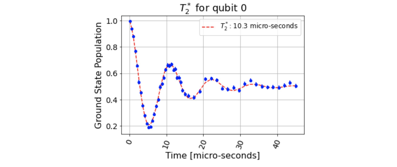
Figure 11.15 – T2* characterization of qubit 0, where T2* is estimated at 10.3 ms

Congratulations! You have just successfully characterized all three decoherence effects on a qubit. Of course, we're not done yet! Characterizing the decoherence of a qubit is important, but equally important is mitigating the errors. In the final section of this chapter, we will review readout errors, which are errors based on the effects of measuring and acquiring the results from the qubits. These readout errors are fairly common on near-term quantum systems, so it is a good tool to have in your development toolbox.

Mitigating readout errors

Ignis has measurement filters that can be used to mitigate various types of errors, such as measurements and tensors.

The measurement calibration is what we will use to mitigate measurement errors in this section. The process begins by first generating a list of circuits, where each circuit represents each of all the possible states of the qubits specified, then executing the circuits on an ideal simulator, the results of which we will then pass into a measurement filter. The measurement filter will then be used to mitigate the measurement errors. In the following example, we will first run the circuits on a simulator without any noise models. Then, we will create a noise model that will be applied to all the qubits of the simulator. Then we will execute the circuits on the noisy backend device, where we will then apply the measurement filter to mitigate the errors as best we can. Finally, we will view the results of the measurement filter and compare them to the original noisy results.

We'll begin by importing the necessary methods and classes from the Ignis mitigation library, specifically the complete_meas_cal method and the CompleteMeasFitter class. The first method, measurement calibration circuits, returns a list of circuits that cover the full Hilbert space of the system. What this means is that if you have n qubits, then all 2n basis states will generate a list of quantum circuits. The second is the complete measurement fitter class, which initializes a measurement calibration matrix based on the list of quantum circuits returned from executing the measurement calibration circuits to generate a measurement correction fitter:

# Import Qiskit classes

from qiskit.providers.aer import noise

from qiskit.tools.visualization import plot_histogram

# Import measurement calibration functions

from qiskit.ignis.mitigation.measurement import complete_meas_cal, CompleteMeasFitter

The parameters for each are as follows:

• complete_meas_cal:

  qubit_list: The list of qubits to execute the measurement correction onto. If no list is provided, then it will execute the measurement correction over all the qubits.

  qr: Quantum registers or the size of the quantum register. If none is specified, then it will create one.

  cr: Classical registers or the size of the classical register. If none is specified, then it will create one.

  circlabel: A label to prefix the circuit name so as to uniquely identify it.

  Returns: This returns two lists. The first is a list of calibration QuantumCircuits., while the second is a list of state labels for each calibration circuit.

• CompleteMeasFitter:

  Results: The list of quantum circuits returned from running the complete_meas_cal method. The class allows you to set the calibration matrix later, so it is not required to construct.

  state_labels: The list of state labels returned from the complete_meas_cal method. The ordering of the state labels will be followed when generating the measurement fitter.

  qubit_list: The list of qubits to apply. If none are specified, then the qubit list will be generated based on the first state label entry, state_labels[0].

  Circlabel: If the qubits had a prefix label in the complete_meas_cal method.

The complete measurement fitter also includes some methods we can use that will allow us to be a bit more flexible when generating our fitter, such as the following:

• add_data(new_results[,…]): This is to add the quantum circuit list results from the complete measurement calibration.
• subset_fitter([qubit_sublist]): Generates a fitter object of a subset from the original qubit list.
• readout_fidelity([label_list]): Generates the readout fidelity of the calibration matrix based on the results from the complete measurement calibration method.

Next, we will generate the complete measurement calibration circuits. We will generate a five-qubit set so that we can use it on any of the five-qubit quantum computers. Then, we will generate the calibration circuits using the complete_meas_cal method with a prefix circuit label, mcal, followed by printing out the number of circuits, which should equal 2n circuits, where n is equal to 5, in this case. Finally, we will draw any of the calibration circuits returned. In this example, we will draw the last one, which represents the value 11111:

# Generate the calibration circuits

# Set the number of qubits

num_qubits = 5

# Set the qubit list to generate the measurement calibration # circuits

qubit_list = [0,1,2,3,4]

# Generate the measurement calibrations circuits and state # labels

meas_calibs, state_labels = complete_meas_cal(qubit_list=qubit_    list, qr=num_qubits, circlabel='mcal')

# Print the number of measurement calibration circuits # generated

print(len(meas_calibs))

# Draw any of the generated calibration circuits, 0-31.

# In this example we will draw the last one.

meas_calibs[31].draw()

The printed result is the total number of calibration circuits, 32, which the complete_meas_cal method produces. This will create 32 circuits where each is initialized according to the state levels, which would run from 00000 through 11111. The following circuit diagram pertains to the last circuit, 11111, as follows:

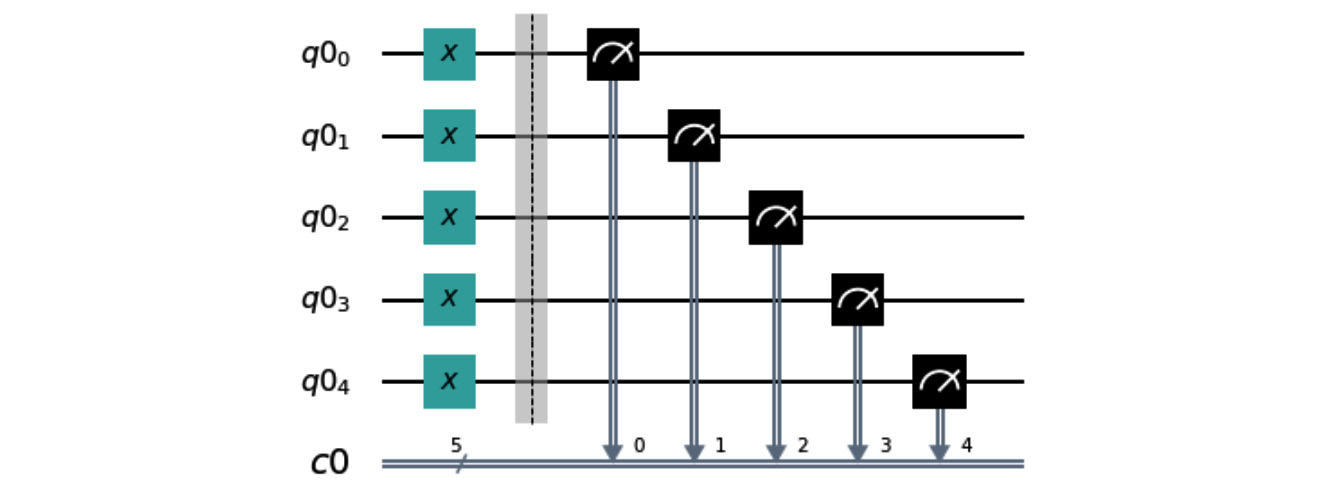
Figure 11.16 – The last calibration circuit, representing value 11111

If you wish to see all the state labels, simply print them out, as follows:

state_labels

This results in listing out all the state labels from 00000 through 11111, which matches the calibration circuit results.

Now that we have our calibration circuits, let's start by first executing it on a simulator so that we can see what an ideal result is, meaning no noise effects or errors. Once we get our results, we will generate the measurement fitter and print out the calibration matrix:

# Execute the calibration circuits without noise on the qasm # simulator

backend = Aer.get_backend('qasm_simulator')

job = execute(meas_calibs, backend=backend, shots=1000)

# Obtain the measurement calibration results

cal_results = job.result()

# The calibration matrix without noise is the identity matrix

meas_fitter = CompleteMeasFitter(cal_results, state_labels, circlabel='mcal')

print(meas_fitter.cal_matrix)

The result is the following calibration matrix, where the rows and columns represent the measured states and the prepared states, respectively:

[[1. 0. 0. ... 0. 0. 0.]

[0. 1. 0. ... 0. 0. 0.]

[0. 0. 1. ... 0. 0. 0.]

...

[0. 0. 0. ... 1. 0. 0.]

[0. 0. 0. ... 0. 1. 0.]

[0. 0. 0. ... 0. 0. 1.]]

Here, the diagonal values are all 1, and all the other fields are 0. This indicates that the measured states correctly match the prepared states.

The measure fitter also includes a nice plot method to visualize the accuracy of the results. To plot the calibration matrix, simply run the following:

meas_fitter.plot_calibration()

The results have a grayscale-based shading, where the darker cells indicate that the accuracy is closer to 1, and the lighter cells indicate accuracy closer to 0, where 1 indicates a 100% match between the measured and prepared states . Due to the default width of the following figure, the states listed across the top of the rendered calibration matrix are difficult to read. However, what it indicates are the prepared states starting with 00000 on the left-most column, increasing along each column towards the final prepared state, 11111:

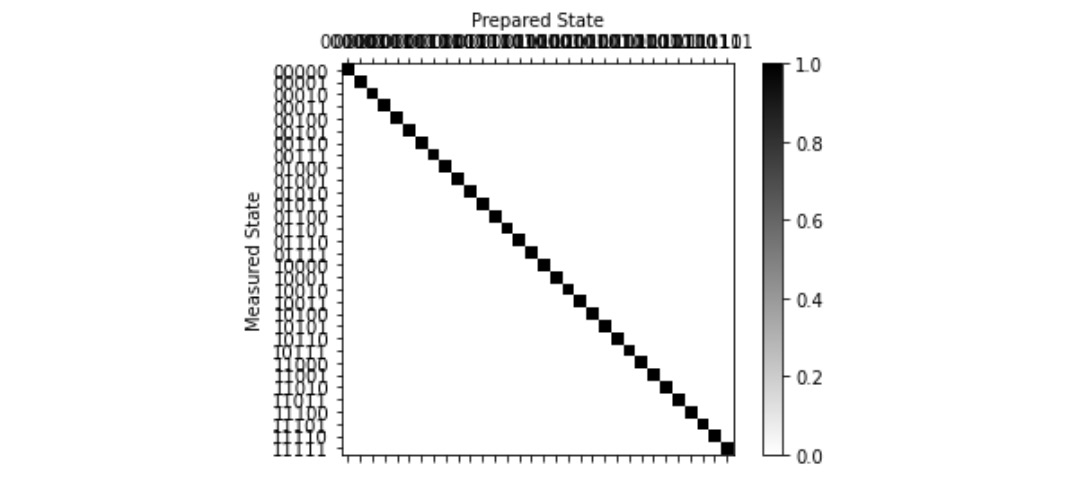
Figure 11.17 – Plot representation of the measured and prepared state results

Now let's run the same steps, but rather than using a simulator, let's run through an actual quantum device. We will start by creating a circuit with five qubits and we'll place one qubit in superposition and entangle it with all the other qubits:

# Create a 5 qubit circuit

qc = QuantumCircuit(5,5)

# Place the first qubit in superposition

qc.h(0)

# Entangle all other qubits together

qc.cx(0, 1)

qc.cx(1, 2)

qc.cx(2, 3)

qc.cx(3, 4)

# Include a barrier just to ease visualization of the circuit

qc.barrier()

# Measure and draw the final circuit

qc.measure([0,1,2,3,4], [0,1,2,3,4])

qc.draw()

This results in the following circuit:

Figure 11.18 – A five-qubit test quantum circuit where all the qubits are entangled with a qubit in superposition

Next, we will get the least busy backend to execute our circuit. We will filter the results to include only backend systems that have greater than or equal to five qubits, not a simulator, and are in operational mode:

# Obtain the least busy backend device, not a simulator

from qiskit.providers.ibmq import least_busy

# Find the least busy operational quantum device with 5 or more # qubits

backend = least_busy(provider.backends(filters=lambda x: x.configuration().n_qubits >= 4 and not x.configuration().simulator and x.status().operational==True))

# Print the least busy backend

print("least busy backend: ", backend)

This results in the least busy device available at the time it was executed. The results will vary based on the devices available to you and their operational state. At the time of writing, the backend result was ibmqx2.

Now that we have our backend, we can execute our circuit as follows:

# Execute the quantum circuit on the backend

job = execute(qc, backend=backend, shots=1024)

results = job.result()

Next, we will extract the result counts from the noisy backend results, which have not yet been mitigated. We will accomplish this by generating the measurement fitter filter, and then we will apply the filter to our backend results. Finally, we will capture the filtered result counts and compare the results between the filtered and non-filtered result counts:

# Results from backend without mitigating the noise

noisy_counts = results.get_counts()

# Obtain the measurement fitter object

measurement_filter = meas_fitter.filter

# Mitigate the results by applying the measurement fitter

filtered_results = measurement_filter.apply(results)

# Get the mitigated result counts

filtered_counts = filtered_results.get_counts(0)

Now, let's plot the noisy results from the backend:

plot_histogram(noisy_counts)

The result of this is the following; you can observe that we have the expected high probability for 00000 and 11111. However, note that there are some very small results that are not part of what is expected. These little results are due to the readout errors from the quantum system:

Figure 11.19 – Results without readout error mitigation

Finally, let's plot the mitigated results from the backend:

plot_histogram(filtered_counts)

The results illustrate how the filters have significantly decreased the errors from the previous noisy results such that only the expected values of 00000 and 11111 are probable, and all the other values have diminished:

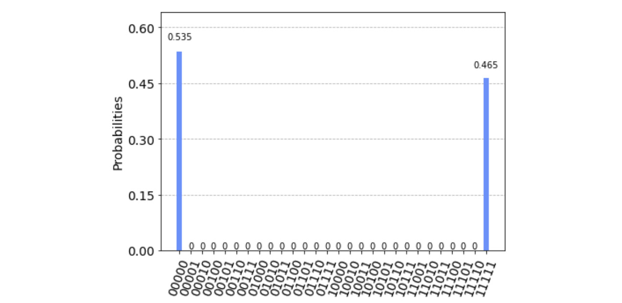
Figure 11.20 – Mitigated results from the backend

Congratulations! You have successfully mitigated noise from a quantum device. Furthermore, you were able to also generate a list of calibration circuits that can be fitted to any number of backend devices.

Summary

In this chapter, we covered some of the many effects that noise has on a quantum computing system. We discovered how we can measure decoherence effects using fitters to help visualize and test the quantum systems and calibrate the readout errors so as to apply error mitigation to the noisy results of a system. Finally, we leveraged the filter to mitigate the noisy results from a quantum device, which significantly reduced the errors.

In the next chapter, we will learn how to create quantum applications using the many features available in Aqua, where we can then look at creating quantum algorithms, and ultimately provide you with all the tools to create your own quantum algorithms and quantum applications.

Questions

1. List the various characterizations of a qubit.
2. Which decoherence is analyzed using the Ramsey experiment?
3. What is the difference between relaxation and dephasing decoherence?
4. Which of the following is not a value for dephasing – T1, T2, or T2*?
5. What is the maximum number of qubits you can apply to a measurement filter?
6. What is the difference between T2 and T2*?
7. What do the rows and columns of a calibration matrix relate to?
8. What is the name of the effect when a qubit decays from the excited state to the ground state?

Further reading

• Sutor, B., Dancing with Qubits, Packt Publishing: https://www.packtpub.com/data/dancing-with-qubits
• Nielsen, M. & Chuang, I., Quantum Computation and Quantum Information, Cambridge University Press: https://www.cambridge.org/us/academic/subjects/physics/quantum-physics-quantum-information-and-quantum-computation/quantum-computation-and-quantum-information-10th-anniversary-edition
• Qiskit Textbook: https://qiskit.org/textbook