Chapter 3: Creating Quantum Circuits using Quantum Lab Notebooks

In this chapter, you will learn how to create circuits using the Quantum Lab Notebooks installed on the IBM Quantum Experience. You will learn how to save, import, and leverage existing circuits without having to install anything on your own computer. This will allow you to get a jump start on developing quantum circuits right away and ensure that you will be able to run the tutorials based on the currently installed version.

The following Quantum Information Science Kit (Qiskit) notebook topics will be covered in this chapter:

• Creating a quantum circuit using Quantum Lab Notebook
• Opening and importing existing Quantum Lab Notebook
• Developing a quantum circuit on Quantum Lab Notebook
• Reviewing results of your quantum circuit on the Quantum Lab Notebook

After completing this chapter, you will be able to leverage the capabilities of the Quantum Lab Notebooks, which will allow you to collaborate with others, share notebooks with others, import notebooks such as those that accompany this book, and run them directly from Quantum Lab. The Qiskit textbook is also capable of running on a Notebook, so as new features are released, you can be assured that you will be able to run them directly from your Notebook.

Technical requirements

In this chapter, some basic knowledge of programming is required, and some Python development is preferred. If you are familiar with other Notebook applications such as Jupyter Notebook then you may want to peruse this chapter, as most of the content here might be familiar to you.

We will not be using much Python-specific code here yet, but there will be some Qiskit code to help get you started in understanding and using the Qiskit Notebook. Here, I will cover the Qiskit basics as we go along, but rest assured we will have plenty of time in Chapter 7, Introducing Qiskit and Its Elements to review the many functions and features of Qiskit. Here is the source code used throughout this book: https://github.com/PacktPublishing/Learn-Quantum-Computing-with-Python-and-IBM-Quantum-Experience.

Here is the link for the CiA videos: https://bit.ly/35o5M80

Creating a quantum circuit using Quantum Lab Notebooks

Quantum Lab Notebooks provided to you via the IBM Quantum Experience platform will help you generate robust experiments that allow you to create quantum circuits and integrate those circuits with classical experiments or applications. Quantum Lab Notebooks generally contain a set of cells that you can use to write, test, and run your code in each cell individually.

You can also include Markdown language in the cells to capture any notes or non-code content, to help keep track of your learning or project. In this section, we will recreate the same quantum circuit you completed in Chapter 2, Circuit Composer – Creating a Quantum Circuit, only this time you will be using the Qiskit Notebook. So, let's get started!

Launching a Notebook from the Quantum Lab

To create a quantum circuit, let's start by launching the Quantum Lab Notebook from the Quantum Lab view. From the left panel under Tools, select Quantum Lab to launch the view, as illustrated in the following screenshot:

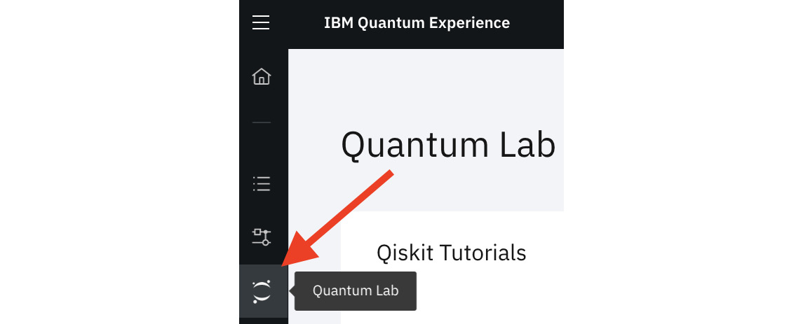
Figure 3.1 – Launching the Quantum Lab view (left panel)

Now that you have the Quantum Lab view open, let's take a look at what each component of the Notebook provides.

Familiarizing yourself with the Quantum Lab components

In this section, we will become familiar with each of the components that make up the Quantum Lab view. As you see in Figure 3.2 (starting from the top section, where you can see there are quick links to the Qiskit tutorials), the quick links are grouped into three sections, as follows:

• The first one is for starters, titled 1_start_here.ipynb. This will review the introductory functions and features of Qiskit.
• The second group contains more advanced level tutorials.
• The third contains tutorials specific to certain fundamentals such as optimization, artificial intelligence, and many other domains.

Under the quick links is the list of all previously saved notebooks. You can choose to open any of those listed, or you can create or import notebooks by selecting either the New Notebook + or Import button respectively, as illustrated in the following screenshot:

Figure 3.2 – Quantum Lab view

In the next step, we will create a new Notebook.

Creating a new Notebook

In this section, we will review the various functionalities available to ensure that you have a good understanding of all the different features available to you.

In the following screenshot, we can see the landing page of the Circuit Composer editor view:

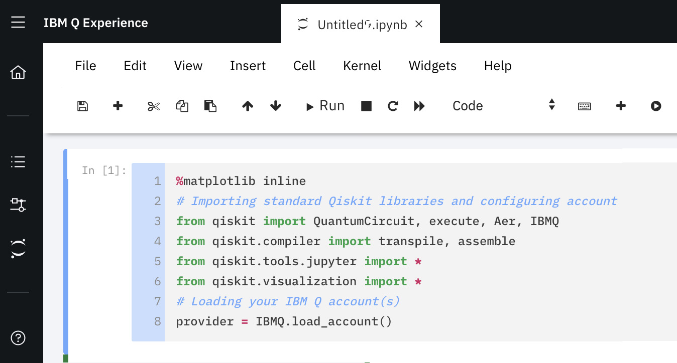
Figure 3.3 – Notebook landing page

The following points provide a description of the functions and features and what they contribute to the creation of a quantum circuit:

• When the Notebook loads up, you'll notice the first cell contains autogenerated code that includes some from Qiskit. Qiskit will be discussed in detail in Chapter 7, Introducing Qiskit and its Elements.

  The autogenerated code functions help to get your code up and running by adding some libraries and objects that are common when creating and running a quantum circuit. We'll review details of these objects further so that you can understand what each line pertains to and what the objects are generally used for.

  Important note

  Note that these may change as new features are added or updated to Qiskit, so the content of these lines may alter over time.

• The following lines of code, which can also be seen in the preceding screenshot, contain the most commonly used objects from the Qiskit library and the code for loading of your account details so that you can connect to the quantum systems.

  This is the first line of the autogenerated code block in your Notebook:

  %matplotlib inline

  The preceding code imports the Matplotlib plotting library, which provides the ability to embed plots and publication quality figures into applications. Details about Matplotlib can be found on their home page here: https://matplotlib.org/

  The next line imports four Qiskit objects that are commonly used to create and run a quantum circuit. QuantumCircuit is used to create a new circuit, which is a list of instructions bound to some registers. execute is an asynchronous call to run a circuit and return a job instance handle. Aer and IBMQ are providers for backend simulators and devices and to manage account details, respectively.

  In the following code snippet, you can see we import each of these from the qiskit package:

  from qiskit import QuantumCircuit, execute, Aer, IBMQ

  transpile and assemble are compiler objects used to translate and compile circuits, while assemble provides a list of circuit schedules, as shown in the following code snippet:

  from qiskit.compiler import transpile, assemble

• The following lines in the autogenerated block of code import all tools and objects from the Jupyter Notebook and visualization libraries, respectively. Jupyter Notebooks is what the Qiskit Notebook is built upon, so it will leverage existing features already familiar to those of you who compose experiments on a Jupyter Notebook.

  These features include creating new files, running kernels, and triggering cells. The visualization library includes many features used to visualize results from experiments such as histograms and bar charts, and in various formats, including Matplotlib, Latex, and so on. The code can be seen here:

  from qiskit.tools.jupyter import *

  %from qiskit.visualization import *

• And finally, the IBMQ.load_account() function loads your account information, particularly the application programming interface (API) token that was assigned to you when you initially registered. This is done if you desire to run an experiment on an actual device; the loading of your API token and other account information needed to run an experiment is already available without any extra work on your part. The following code snippet shows this:

  provider = IBMQ.load_account()

  This way, the content of your experiment is not cluttered with information that is not relevant to your experiment and conclusions.

Now that we are familiar with the autogenerated code, we'll take a quick look at the Qiskit Notebook itself. You'll note that its layout is very similar to that of a Jupyter Notebook, so those who are already familiar with Jupyter Notebooks will undoubtedly recognize the layout.

Learning about the Qiskit Notebook

For those who are new to the Qiskit Notebook, there are a couple of things to note that will help you understand how coding and running your code work. Those of you who are already familiar with Jupyter Notebooks can skip this section.

The Quantum Lab Notebooks run code one cell at a time. As shown in the following screenshot, a cell is a section of the Notebook that can contain text, metadata, and source code, such that it encapsulates the autogenerated code we looked at earlier. It simplifies coding by breaking up the code into these cells. The cells can be run individually by selecting the cell with your mouse and clicking the Run button, as illustrated in the following screenshot:

Figure 3.4 – Notebook cell and operations

From the preceding screenshot, in the top row of the Qiskit Notebook menu options you will see some usual operations you would find in a typical document editor, as follows:

• File: Save, Checkpoint, Print Preview, Close, and Halt
• Edit: Modify Cells, Move Cells, Merge Cells, and so on
• View: Toggle Headers, Toolbars, and other views
• Insert: Insert cells above or below selected cell
• Cell: Run cell, run all cells, and more
• Help: Provides support content

There is one specific operation in the Notebooks menu list to take note of, and that is the Kernel. For those of you with an existing version(s) of Python, do take note that Qiskit, at the time of this writing, is running on Python version 3.

To confirm this, you can select Kernel from the drop-down menu and note that there is a Change Kernel option. You will see Python 3 as the only option. However, if you install Qiskit on your local machine that contains other versions of Python, you might see them listed here as well. I mention this so as to ensure you have the correct kernel selected to run Qiskit experiments. Otherwise, you may encounter some errors due to version incompatibility.

Another thing to note is related to the various different formats in which you can download a Qiskit Notebook. By selecting the File | Download as option you will see the various formats, as shown in the following screenshot:

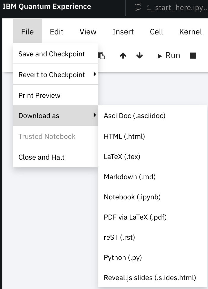
Figure 3.5 – Download formatting options

Up to now, you should be familiar with the functionality and features available on the Qiskit Notebook. These are features that make it easy to share experiments and make quick changes to them. We can now start creating and running quantum experiments on our notebooks using Qiskit.

Opening and importing existing Quantum Lab Notebook

Oftentimes, we wish to share our experiments with others and run others' experiments ourselves. Importing a Qiskit Notebook is easy in that the Quantum Lab home page has a link to Import button, next to the New Notebook + button, as shown in the following screenshot:

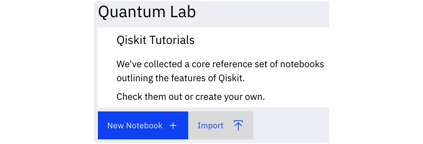
Figure 3.6 – Quantum Lab home page

This will launch your machine's file dialog to select the Qiskit Notebook you wish to import into your workspace on IBM Quantum Experience (IQX). To open an existing Qiskit Notebook, or one you have just imported, simply go back to your Qiskit Notebook page and select the Notebook you wish to open from the file list at the bottom of the view, as illustrated in the following screenshot:

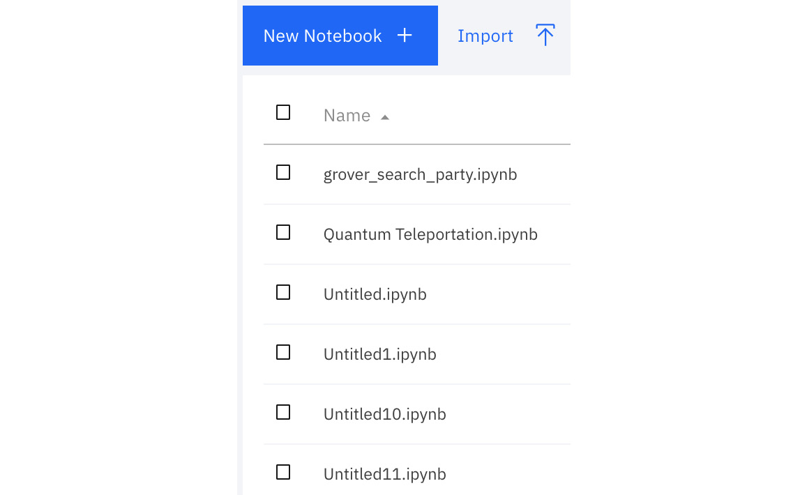
Figure 3.7 – List of previously opened notebooks

Now that you are familiar with the Notebooks and the autogenerated code, let's quickly create the same circuit we generated in the previous chapter, only this time we will create it using only the Notebook.

Developing a quantum circuit on Quantum Lab Notebooks

Let's take a quick look at the quantum circuit we created in the previous chapter. For convenience, the circuit is given as follows:

Figure 3.8 – Quantum circuit previously created using the Circuit Composer

The preceding circuit comprises of two gates—Hadamard and Controlled-Not—and two measurement operations on 2 qubits, respectively. This circuit was very easily constructed on the Circuit Composer; however, as we learn more about quantum circuits and begin to work on more complicated algorithms and circuits, it will be difficult to leverage a user interface such as the Circuit Composer. So, we will code the construction of quantum circuits and algorithms as we move forward instead.

To create the previous quantum circuit on a Notebook, follow these steps:

1. From the Quantum Lab Notebook, create a new Notebook and enter the following code in an empty cell:

   qc = QuantumCircuit(2,2)

   qc.h(0)

   qc.cx(0, 1)

   The preceding code creates QuantumCircuit. The two parameters pertain to the number of quantum bits (qubits) and classic bits we want to create, respectively. In this example, we will create two of each.

   The second line adds a Hadamard gate onto the first qubit. Note that the index values of the qubits are 0 based. The third line adds a Controlled-Not gate that entangles the first qubit (q0) as the control to the second qubit (q1), the target. The parameters in the function pertain to the control and target, respectively.

2. Now, select Run to run the cell. Once the cell has completed running, you should see the output display InstructionSet of the results and a new cell generated below the one you just ran, as shown in the preceding code snippet. InstructionSet is a class of instruction collections and their contexts (classic and quantum arguments), where each context is stored separately per each instruction.

   Here is the output we are given after running the preceding code:

   <qiskit.circuit.instructionset.InstructionSet at 0x7fc632176eb8>

3. Next, we will add the measurement operators to our circuit so that we can observe our results classically. Notice in the following code snippet that we are using the range method so as to simplify the mapping of each qubit to its respective classic bit:

   qc.measure(range(2), range(2))

4. Run the preceding cell to include the measurement operators to our circuit. Now that we have created the circuit and included the same gates and operations we did in Chapter 2, Circuit Composer – Creating a Quantum Circuit, let's draw the circuit and compare. Draw the circuit using the draw function, shown as follows:

   qc.draw()

   You should now see the following results, after the draw method is complete:

Figure 3.9 – Rendered image of the quantum circuit

Notice that the preceding circuit is identical to that which you created earlier. The only difference is the initial number of qubits. The Circuit Composer defaults to 5 qubits, whereas here we specified only 2. The circuit will run the same, both on the simulator and on an actual quantum device, since we are only using 2 qubits.

In this section, we have learned to navigate the Quantum Lab Notebook. We also learned how to open an existing Notebook, along with opening, creating, and importing the Notebook. We also saw how to develop a quantum circuit.

Now, we will move on to review the results of the quantum circuit.

Reviewing the results of your quantum circuit on Quantum Lab Notebooks

In this section, we'll conclude this chapter by running the circuit on a quantum simulator and a real device. We'll then review the results by following these steps:

1. From the open Notebook, enter and run the following in the next empty cell:

   backend = Aer.get_backend('qasm_simulator')

   The preceding code generates a backend object that will connect to the specified simulator or device. In this case, we are generating a backend object linked to the QASM simulator.

2. In the next empty cell, let's run the execute function. This function takes in three parameters—the circuit we wish to run, the backend we want to run it on, and how many shots we wish to execute. The returned object will be a job object with the contents of the executed circuit on the backend. The code for this can be seen here:

   job_simulator = execute(qc, backend, shots=1024)

3. We now want to extract the results from the job object. In order to do that, we will call the result function, illustrated as follows, and save it in a new variable:

   result_simulator = job_simulator.result()

4. Since we ran our experiment with 1024 shots, we want to get the results from the counts. In order to do that, we can call the get_counts() method by passing in our circuit as the argument. Once we receive the counts, let's print out the results by running the following code:

   counts = result_simulator.get_counts(qc)

   print(counts)

   Note that the count results, shown as follows, may be different from your count results, which are based on the randomness of the qubits. But overall, the results will be similar by approximately 50%:

   

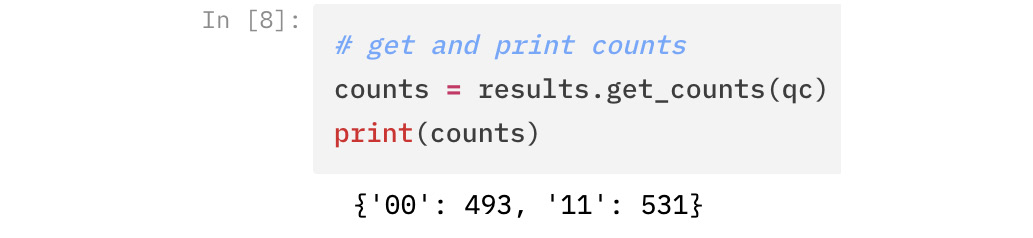
   Figure 3.10 – Count results from the quantum circuit

5. Finally, let's visualize the result counts by plotting them using a histogram. We'll first import the plot_histogram method from the qiskit.visualization library and pass our counts in as an argument, as follows:

   from qiskit.visualization import plot_histogram

   plot_histogram(counts)

   As you can see in the following screenshot, the results are very similar to our results from the Circuit Composer in that 50% of the time our results are 00, and the other half of the time they are 11:

Figure 3.11 – Histogram view of the count results

Now that we have run our quantum circuit on a simulator, let's run this same quantum circuit on a real quantum computer.

Executing a quantum circuit on a quantum computer

To run this quantum circuit on a quantum device, we will continue with the following steps:

1. The only change you need to update in the steps from the preceding section is to go from running on a simulator to a real device in Step 1 from the previous steps, which is where you specify the name of the backend. In Step 1, we set the backend to the qasm_simulator. In this step, we will update to an actual device. So, let's first get a list of backends from our providers by running the following code in a new cell:

   provider.backends()

   The preceding method will return a list of all the simulators and real devices currently available to you, shown as follows. Note that the devices listed may change over time, so the results shown may be different when you run the method:

   

   Figure 3.12 – List of available quantum computers (quantum devices)

2. The only change you need to update from the steps in the previous section is to specify which quantum computer from the list of backend devices you wish to run the experiment. In the previous steps, we set the backend to the qasm_simulator, whereas in this step we will update our backend to use a real device from the list. In this case, we'll choose ibmq_vigo. This list may appear different to you, so pick one from your list if ibmq_vigo is not listed. To do this, run the following code in a new cell:

   backend = provider.get_backend('ibmq_vigo')

   The preceding code assigns the ibmq_vigo quantum computer as our backend.

3. From the previous steps, repeat Step 2 to Step 5 to run the circuit on a real device. Your results will seem a little different. Rather than just the 00 and 11 results, you will see that there are some 01 and 10 results, shown in the screenshot that follows, albeit only a small percentage of the time.

   This is due to noise from the real device, which is why they are often referred to as Noisy Intermediate-Scale Quantum (NISQ) systems or near-term devices. The noise can come from an array of things, such as ambient noise and decoherence. Details about the different types of noise and their effects will be discussed in detail in Chapter 11, Mitigating Quantum Errors Using Ignis.

   The results can be seen in the following screenshot:

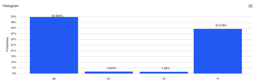
Figure 3.13 – Histogram plot of results

Congratulations! You have just completed running a quantum circuit on both a quantum simulator and a real quantum device using the Quantum Lab Notebooks. As you can see, by using the Notebook you can use many built-in Qiskit methods to create circuits and run them on various machines with a simple line of code, whereas on the Circuit Composer you would have to make various changes that would take a lot of time to complete.

Summary

In this chapter, you learned about the Quantum Lab Notebooks and ran a simple quantum circuit. You completed three basic functional steps: creating a quantum circuit using the Notebook and the Qiskit library, executing your circuit with a backend simulator and real device, and reviewing and visualizing your results from within the Notebook.

One thing you might have noticed is that using the Notebook with Qiskit also simplifies integrating your classical experiments with a quantum system. This has provided you with the skills and understanding to enhance your current Python experiments and run certain calculations on a quantum system, making them a hybrid classical/quantum experiment.

When the quantum calculations have completed, the results can be very easily used by your classical experiments.

Now that we are familiar with the Quantum Lab Notebooks and are able to create and execute a circuit, in the next chapter, we will start learning the basics of quantum computing and the quantum mechanical principles of superposition, entanglement, and interference.

Questions

1. Quantum Lab notebooks are built upon which application editor?
2. How would you create a 5-qubit circuit, as we did in Chapter 2, Circuit Composer - Creating a Quantum Circuit?
3. To run the experiment on another real device, which quantum computer would you select if your quantum circuit has more than 5 qubits?
4. When you run on a real device, can you explain why you get extra values when compared to running on a simulator?