7. Introducing Facility Fixed and Variable Costs

This chapter discusses the costs of facilities. We will model these costs in two categories: fixed and variable. They can be applied to plants and warehouses.

The fixed costs are a one-time charge independent of the volume. This could be the cost of building the site; expanding the site; adding equipment to the site like extra lines or equipment in plants, additional racking or automation in warehouses; paying taxes; or staffing the location. The fixed cost could be thought of as a one-time capital investment or as an annual fixed operating cost. Capital investments are treated differently than fixed operating costs because they are depreciated over time and you do not necessarily need to justify the investment over a single year. Fixed operating costs represent costs that are incurred during the normal operation of the plant, line, or warehouse. In essence, these are costs that are incurred each year (or month) independent of how much volume is handled at the facility. We will discuss this topic later in the chapter.

The variable costs are those that depend on the actual number of units that are made at a facility or that pass through a facility. That is, to determine the total variable cost, you simply multiply the total units that are made at a facility or that pass through a facility by the variable cost. For example, if the variable cost of production is $2, then every unit adds $2 of cost. Note that different products may have different characteristics, for example different sizes, weights, or manufacturing requirements. In this case, you may use a simple conversion table to convert units to another measure before applying the variable cost.

In practice, there is no correct answer on what cost is “fixed” and what cost is “variable.” One of the authors of this book was told by two vice presidents of supply chain from two different firms in the same week the following:

1. “There is no such thing as fixed costs. All my costs are variable over time. I can change anything.”

2. “There is no such thing as a variable cost. All my costs are fixed. After I open a warehouse, I have to fully staff it and cannot adjust that in any way that impacts my current budget.”

Both views are valid and you can take either view when setting up your supply chain model. It is important to understand how these costs work to determine how you want to use them in your supply chain. Also, remember that we are not necessarily interested in the accounting definitions, but, instead, we want to use these costs in the way that makes the most sense for the types of decisions we want to get out of the model.

Let’s look at the two extreme cases to understand how the costs work:

If you model all the costs at a facility as fixed, then the optimization has the incentive to minimize the number of facilities it opens (to minimize the total fixed cost) and, when a facility is open, it will focus on maximizing the amount of product put through that facility (which is why you may want to include capacity constraints).

If you model all the costs at a facility as variable, then the optimization has an incentive to use the facilities with the lowest variable cost (as long as extra transportation costs don’t outweigh it) and no incentive to avoid adding additional facilities (so the model may choose to use many different facilities unless you limit the number of facilities with a constraint).

You should note that there are some advanced varieties of the fixed and variable costs that allow you to capture other details within the supply chain.

First, you can think about the fixed costs as a step function. That is, instead of just a single fixed cost, you may have several fixed costs you need to add, depending on how much product flows through or is made at the facility. For example, if you open a plant with one shift, you may have a fixed cost of $5 million. If you add a second shift, your fixed costs go up to $6 million but it gives you additional capacity. And if you add a third shift, costs go up to $7 million with the added capacity. This seems like a combination of a fixed and a variable cost, but in reality, it behaves like a fixed cost. The model will open it up for a particular size, and after it does, all things being equal, it has an incentive to then use as much of the available capacity as possible.

Second, you can think about the variable costs depending on the size of the facility, or the economies of scale. That is, as a facility gets larger, the cost per unit may go down. You capture this again with the step sizes and simply have a lower variable cost for each step size. For example, if you open up a warehouse with the capability to process 200,000 pallets a year, your cost may be $5 per pallet. If the facility can process 400,000 pallets per year, your variable costs may drop to $4.50 per pallet. Often, to prevent the model from opening the 400,000-pallet facility and using it for only 100,000 pallets’ worth of product, you either model a fixed cost in addition to the variable cost or enforce a minimum flow through the facility. That is, you stipulate that you would have to send at least 200,001 pallets through the larger facility before you would even consider using it.

In the math formulation section that follows, you’ll see how the fixed and variable costs balance against each other. And you will see how the use of options can allow you to capture the step functions in the fixed and variable costs.

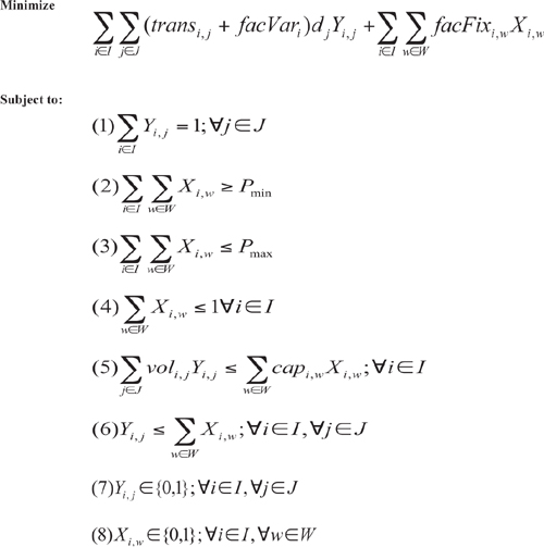
This model is quite similar to those we have discussed previously. We have added a few new concepts:

• The set W represents the set of facility options. Each option represents a different sizing decision for the same physical location. That is to say, if you have the choice between building a small, medium, or large warehouse at each potential site, then W would contain three entries. This set of options now allows us to model changes in fixed and variable costs for each option. To keep the formulation simple, we are showing only the change in fixed costs with the options, but the model can be extended to include the change in variable costs.

• The decision on whether to open a facility has been generalized to include the choice of facility option. That is, variable X_i,w will be set to 1 if and only if facility i is opened with option w. Note that constraint (4) ensures that you don’t select more than one facility option for each facility that is opened. For example, constraint (4) forces you to pick the small, medium, or large warehouse option, not all three or any two.

• We have added facility fixed (facFix) and variable costs (facVar) to the objective function. Now these costs are added to the transportation costs. So the optimization will consider all the costs. The optimization will want to incur a fixed cost only if it absolutely needs the capacity or if the savings from the variable or transportation costs make it worthwhile.

• We have also added limits to the capacity of a facility. This is captured in constraint (5). If you have fixed costs and no capacity constraints, the model may be tempted to open as few facilities as possible and send unrealistically high volumes through these facilities.

• Note that our model now allows the solver engine to determine how many facilities to open. Constraints (2) and (3) restrict the total number of opened facilities to be between P_min and P_max. Without facility fixed costs, there would have been no disincentive for our model to simply open all facilities.

Let’s continue our case from the preceding chapter by adding variable costs to the model. In this case, the firm estimates that they pay $2.75 per package that they handle in the Louisville facility. If we simply add this to the baseline, we add $9.0 million in variable warehouse costs to the $16.6 million in transportation costs. The total cost is now $25.6 million. Because the Louisville facility is older, the firm believes that the variable costs will drop to $2.50 per package in a new location.

When we run the model, the solution is not the same as the run without the variable costs. The three locations are the same (Louisville, Kentucky; Fresno, California; and Dover, Delaware), but the territories have shifted. When you look at the map shown in Figure 7.1, you see that Dover’s territory has expanded (compare back to Figure 6.12). It has picked up more territory on the East Coast and Florida and some regions around Wisconsin and Texas.

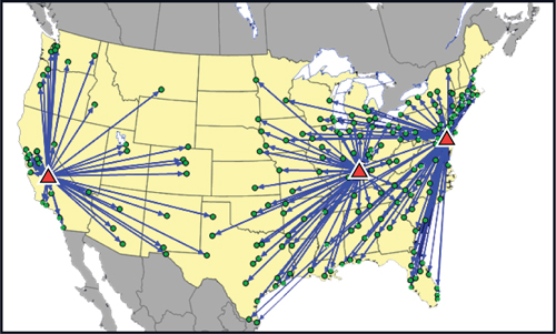
Figure 7.1. Revised Outbound Distribution Solution with Variable Costs Added

Why has this happened?

The objective function considers both the transportation costs and the variable costs. It does not consider distance to the customer. Also remember from Chapter 6, “Adding Outbound Transportation to the Model,” that transportation rates may be relatively flat and not directly correlated with distance. And, with small-parcel rates, you may have a lot of rates that are exactly the same even though the distance from the warehouse is different. Then, the lower variable cost at Dover will push the assignment to that location. If the variable cost difference were even higher, the Louisville facility would have an even smaller territory.

So when the variable cost is different between locations, the decision can change and it can impact your model. Now, the model is making a more nuanced trade-off. All things being equal, the model will move more volume to the low-cost warehouses. When the optimization decides to move more volume to these low-cost locations, transportation costs will rise (or, best case, stay the same), but the overall result is a lower cost.

Determining the variable costs in a model is not always straightforward.

In some cases, especially when you use third-party warehousing or manufacturing, you will have a simple variable cost to include. That is, you will know what the third-party firm charges you per unit produced or handled.

When the facilities are your own, however, you may need to consider the following elements when determining the variable costs:

• Labor Costs—This is the most obvious factor. If you don’t model labor as a fixed cost, you need to determine the labor needed per unit. Firms may have an estimate of this. Some firms may use the very detailed Activity Based Costing methods to determine how much labor cost is incurred for each unit produced or handled. In any case, you need to include both direct and indirect labor.

• Utility Costs—Depending on the type of firm, and more true for manufacturing firms, the more product that moves through a facility, the more electricity and water the facility uses.

• Material Costs—In manufacturing, you will need to purchase additional material for each unit produced or consume packaging material in a warehouse.

Often, it is easier and cleaner to break out the costs by major activity to help quantify the costs. For example, in the warehouse, you may have separate costs for putting product away, for storing the product, and for picking and shipping the product to customers. In the plant, you may break out the costs between making the product and packing it.

When you have many different sites and there is complexity in breaking out the variable costs, a regression analysis can be used. In this case, the total cost of the site is the dependent variable, and the total throughput of the site is the independent variable. You can add other independent variables as the situation requires, such as product type or type of facility. But using throughput can provide helpful insight. When the regression runs, the slope of the line provides information on the variable cost. The y-intercept of the regression can provide insight into your overall fixed cost per facility.

As you can tell, there are many ways to break out the variable costs and each situation is unique. We do recommend that you start with a simple approach and then add sophistication as needed.

In summary, when you run a scenario with one more facility allowed than another scenario, the difference in cost is the fixed cost threshold. For example, if a model comes back with a four-facility solution at a cost of $10.8 million and the five facility solution is $9.1 million, then the cost of the extra warehouse needs to be less than $1.7 million.

This technique can be a great way to account for fixed costs in a model. This is especially true when making warehouse location decisions. A firm will have a good estimate on the cost of a warehouse and will just need to understand the threshold of adding facilities.

This technique is also powerful when a firm uses third-party warehouses. In these arrangements, the firm may pay only a variable cost to use the third-party facility. This does not mean that the true fixed cost is zero. It reminds us to think deeply about the fixed costs and how we will analyze our results. Each additional warehouse we add to the model increases the amount of management overhead, decreases our control over the supply chain, possibly increases the amount of inventory, potentially erodes our ability to replenish the warehouses with full truckloads, and may cause our suppliers to increase costs if they have to ship into multiple facilities. So it may be impossible or too expensive to estimate these fixed costs. But, again, the management team should be able to judge whether the savings from adding an additional warehouse likely outweigh these hidden costs. For example, if the transportation savings are five times higher than the entire management overhead costs, it is likely that hidden costs will not materially impact our savings.

Having covered the reasons for not including a fixed cost, there are reasons you may want to include fixed costs. These include the following:

• The fixed costs vary significantly from location to location.

• Capacity is an important consideration and you want to model multiple options. For example, you may staff a facility with one, two, or three shifts and the shifts are best treated as fixed costs.

• We need to address capital investment decisions to expand or improve existing locations or open new sites. When considering a capital investment as a fixed cost, you want to be careful to make sure you put the investment in the same time frame as other costs. So if you have an annual model (and therefore your transportation and variable costs are annual numbers), you want to annualize your capital investment so that there is a fair comparison of costs. Most firms follow accounting guidelines in allocating capital investment to a year.

The fixed-operating costs most often include items like the management of the facility, the cost to upkeep the building, the utilities (if not dependent on the number of units you flow through the facility), the number of shifts (if these are not modeled as variable costs), and the taxes on the building and land.

The fixed capital costs include investment costs like building the facility, adding lines, and adding equipment.

It is usually important to separate the fixed operating and fixed capital costs into two distinct buckets.

When you build your business case for implementing one of the results from your network modeling exercise, you often need to financially justify your decision with a net present value (NPV) calculation. In general, the NPV calculation treats the capital investment as a one-time investment at the start of the project. So it is treated separately from the other fixed costs. We have an example of this in the end-of-chapter questions.

To make good decisions about the structure of our supply chain, we may need information on the fixed and variable costs. The accounting systems may just report on total costs. These same systems may attempt to break out fixed and variable costs, but each location in the supply chain may categorize things differently.

One method we have found successful is to look at a firm’s detailed list of expense categories for a facility. This list may contain things like direct labor, overtime, maintenance labor, management, security, IT spend, electricity, and many other expense categories. These are the standard expenses that the accounting team tracks and reports on every month. From this list, the supply chain team, working with the finance, accounting, and other functional areas, goes through the list, item by item, and categorizes each cost into the percent fixed and percent variable. This then provides a standard way to use the accounting data for supply chain design work. For example, the electricity costs may be split 30/70 between fixed and variable. The idea is that some expenses are fixed (because you just have to keep the lights on) and some are variable (the more you process, the more electricity you need to run your machines).

As an example of this process, we worked with a client who had five plants making the same type of product. They had one plant that, according to their accounting systems, cost about 75% more than their other plants. They wanted to justify closing this plant. However, this company sold a very heavy product (and thus expensive to ship) and this plant was located very close to customers. After doing a detailed study using the process we described previously, we determined that this plant was actually very good at making one type of product and very bad at making the other type. When we ran the optimization, the results suggested not only keeping the plant, but actually increasing its production. In the current situation, the plant was making about 50% of each product type. Because the plant was very good at making one type of product and was close to the market, the optimization had that plant make much more of that product and hardly any of the product that it wasn’t good at making. In the end, it made more total product at a much lower cost. The accounting system was failing them because it was reporting on averages. The analysis revealed the underlying cost structure and the optimization model was able to take advantage of that.

When you’re modeling fixed and variable costs, it is important to think about them in the context of your model. The accounting definitions of these terms may not help you make the correct decisions.

For fixed costs, you need to be careful to separate the ongoing fixed costs (like keeping the lights on) from the one-time investments (like building a new building). For the latter, the one-time investments, you need to make sure you put the costs in the same units of time as the other cost elements in your model or you will not get realistic results.

2. If it costs $10 million to build a new facility and you expect to depreciate the building over 20 years, why wouldn’t you include the full $10 million when you are building a model with a year’s worth of demand?

3. Open the file Warehouse Costs by Throughput.xls located on the book Web site. This file contains the total cost to operate different warehouses by throughput. Run a regression analysis and estimate the fixed and variable cost formula. Why might this approach work well for a firm with many warehouses and not very well for a firm with only a few warehouses?

4. A large CPG manufacturer initiated a network study to optimize its manufacturing network to determine where add a line to make a new product. The company had an existing plant in the U.S. it could expand and was considering new locations for the line in either in Mexico or Panama. The costs for the three scenarios are shown in Figure 7.2. The fixed cost for the new line is shown in millions of dollars. The cost of the product, the freight cost, and the duty costs are shown in terms of a cost per unit. The freight cost is the cost to get the product from the production source to the U.S. Distribution Center (DC).

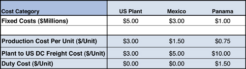
Figure 7.2. Data Used in Analysis

The total demand for the line product is 200,000 units.

When the model was run, the 200,000 units were made in Panama. The company was expecting production to stay in the U.S. because of the high transportation cost from Panama. Use the cost data provided to figure out why Panama was picked.

5. Open the Investment Decisions.zip located on the book Web site. The file contains more details on the model. This is a firm that has five plants around the country and is facing tremendous growth. They have an opportunity to invest in additional capacity and also replace older equipment with much faster equipment. In this case, the investment decisions can be thought of as a step-function of fixed costs. That is, they can add blocks of capacity at a time for a fixed cost.

a. What year will they run out of capacity with their existing network?

b. In Year 5, what is the optimal plan? How would you describe the solution?

c. In Year 5, what other alternative scenarios should they consider?

6. You have completed a study and have found that you can save $7.5 million in the first year after closing two warehouses, opening a new plant, and serving your customers from different facilities. This study was done with one year’s worth of data. The $7.5 million does not include the initial investment to close the warehouses and open the new plant. The initial investment is estimated to be $20 million. For the company you work for, you must include the net present value calculation when you present the business case. For the NPV calculations, your firm uses a 15% interest rate and goes out only five years (the thinking is that too much changes in five years, and they prefer shorter paybacks).

a. Calculate the NPV using the preceding data. Assume the same $7.5 million savings per year. Based on the NPV results, is this a good project?

b. The firm is growing fast. They would assume that the savings grow 5% per year. That is, if they implement this solution, the savings in Year 2 will be 5% higher than the $7.5 million because they will be shipping much more product two years out. What is the new NPV?

c. Being conservative and going back to the original assumptions, how large would the initial investment have to be for the NPV to equal $0 (zero)? How should the firm use this answer to decide whether they should implement this solution?

d. If you had included the full $20 million as a fixed cost in the model, why would the model not have recommended closing the two warehouses and opening the new plant?

7. Open the file Accounting Allocations.xls located on the book Web site to see a list of sample accounts that a firm has for their various plants. Your team has already gone through these accounts and has determined whether the costs are fixed or variable. What are the fixed and variable costs you should load into the model based on this analysis? Which plant has the highest overall fixed cost? Which plant has the lowest per-unit variable cost? How would you rank the competitiveness of these plants?