Chapter 8. Training Models
“Ask not for a lighter burden, but for broader shoulders.”
—Jewish proverb
While the supply of impressive models and data will continue to grow and overflow, it’s reasonable that you’ll want to do more than just consume TensorFlow.js models. You’ll come up with the idea that’s never been done before, and there won’t be an off-the-shelf option that day. It’s time for you to train your own model.
Yes, this is the task where the best minds in the world compete. While libraries could be written about the math, strategy, and methodology of training models, a core understanding will be vital. It’s crucial that you become familiar with the basic concepts and benefits of training a model with TensorFlow.js to take full advantage of the framework.
We will:
-
Train your first model in JavaScript code
-
Advance your understanding of model architecture
-
Review how to keep track of status during training
-
Cover some fundamental concepts of training
When you finish this chapter, you’ll be armed with a few ways of training a model and a better understanding of the process of using data to make a machine learning solution.
Training 101
It’s time to peel back the magic and train a model with JavaScript. While Teachable Machine is a great tool, it’s limited. To really empower machine learning, you’re going to have to identify the problem you want to solve and then teach a machine to find the patterns for a solution. To do this, we’ll view a problem through the eyes of data.
Take a look at this example of information, and before writing a line of code, see if you can identify the correlation between these numbers. You have a function f that takes a single number and returns a single number. Here’s the data:
-
Given –1, the result is –4.
-
Given 0, the result is –2.
-
Given 1, the result is 0.
-
Given 2, the result is 2.
-
Given 3, the result is 4.
-
Given 4, the result is 6.
Can you identify what the answer for 5 would be? Can you extrapolate the solution for 10? Take a moment to evaluate the data before moving on. Some of you might have found the solution: Answer = 2x – 2.
The function f is a simple line, as shown in Figure 8-1. Knowing that, you can quickly solve for an input of 10 and find it would yield 18.
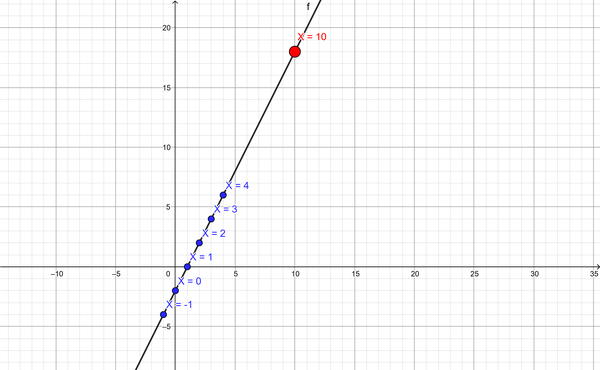
Figure 8-1. X = 10 means Y = 18
Solving this problem from the given data is exactly what machine learning can do. Let’s prep and train a TensorFlow.js model to solve this simple problem.
To apply supervised learning, you’ll need to do the following:
-
Gather your data (both input and desired solution).
-
Create and design a model architecture.
-
Identify how a model should learn and measure error.
-
Task the model with training and for how long.
Data Prep
To prep a machine, you’ll write the code to supply the input tensors, aka the values [-1, 0, 1, 2, 3, 4] and their corresponding answers [-4, -2, 0, 2, 4, 6]. The index of the question has to match the index of the expected answer, which makes sense when you think about it. Since we are giving the model all the answers to the values, that is what makes this a supervised learning problem.
In this situation, the training set is six examples. Rarely would machine learning be used on such a small amount of data, but the problem is relatively small and straightforward. As you can see, none of the training data has been reserved for testing the model. Fortunately, you can try the model because you know the formula that was used to create the data in the first place. If you’re unfamiliar with the definitions of training and testing datasets, please review “Common AI/ML Terminology” in Chapter 1.
Design a Model
The idea of designing a model might sound tedious, but the honest answer is that it’s a mix of theory, trial, and error. Models can be trained for hours or even weeks before the designers of that model understand the performance of the architecture. An entire field of study could be dedicated to model design. The Layers models you’ll be creating for this book will give you an excellent foundation.
The easiest way to design a model is to use the TensorFlow.js Layers API, which is a high-level API that allows you to define each layer in sequential order. In fact, to start your model, you’ll begin with the code tf.sequential();. You might hear this called the “Keras API” due to the origin of this style of model definition.
The model you’ll create to solve the simple problem you are trying to tackle will have only a single layer and a single neuron. This makes sense when you think about the formula for a line; it’s not a very complex equation.
Note
When you’re familiar with the basic equations of a dense network, it becomes amazingly apparent why a single neuron would work in this case, because the formula for a line is y = mx + b and the formula for an artificial neuron is y = Wx + b.
To add a layer to the model, you will use model.add and then define your layer. With the Layers API, each layer that gets added defines itself and automatically gets connected depending on the order of model.add calls, just like pushing to an array. You’ll define the expected input for your model in the first layer, and the final layer that you add will define the output of your model (see Example 8-1).
Example 8-1. Building a hypothetical model
model.add(ALayer)model.add(BLayer)model.add(CLayer)// Currently, model is [ALayer, BLayer, CLayer]
The model in Example 8-1 would have three layers. ALayer would be tasked with identifying the expected model input and itself. BLayer doesn’t need to identify its input because it is inferred that the input would be ALayer. Therefore, BLayer only needs to define itself. CLayer would identify itself, and because it is last, this identifies the model’s output.
Let’s get back to the model you’re trying to code. The architected model goal for the current problem has only one layer with one neuron. When you code that single layer, you’ll be defining your input and your output.
// The entire inner workings of the modelmodel.add(tf.layers.dense({inputShape:1,// one value 1D tensorunits:1// one neuron - output tensor}));
The result is a straightforward neural network. When graphed, the network has two nodes (see Figure 8-2).

Figure 8-2. One input and one output
Generally, layers have more artificial neurons (graph nodes) but also are more complicated and have other properties to configure.
Identify Learning Metrics
Next, you’ll need to tell your model how to identify progress and how it can be better. These concepts aren’t foreign; they just seem strange in software.
Every time I try to aim a laser pointer at something, I generally miss it. However, I can see I’m a bit off to the left or right, and I adjust. Machine learning does the same thing. It might start randomly, but the algorithm corrects itself, and it needs to know how you want it to do that. A method that most fits my laser pointer example would be gradient descent. The smoothest iterative way to optimize the laser pointer is a method called stochastic gradient descent. That’s what we’ll use in this case because it works well, and it sounds pretty cool for your next dinner party.
As for measuring error, you might think a simple “right” and “wrong” would work, but there’s a significant difference between being a couple of decimals off versus being wrong by thousands. For this reason, you generally rely on a loss function to help you identify how wrong an AI is with a predicted guess. There are lots of ways to measure error, but in this case, mean squared error (MSE) is a great measurement. For those who need to know the mathematics, MSE is the average squared difference between the estimated values (y) and the actual value (y with a little hat). Feel free to ignore this next bit, as the framework is calculating it for you, but if you’re familiar with common mathematical notation, this can be represented like so:
Why would you like this formula over something simple like distance from the original answer? There are some mathematical benefits baked into MSE that help incorporate variance and bias as positive error scores. Without getting too deep into statistics, it’s one of the most common loss functions for solving for lines that fit data.
Tip
Stochastic gradient descent and mean squared error reek of mathematical origins that do little to tell a pragmatic developer their purpose. In situations like these, it’s best to absorb these terms for what they are, and if you’re feeling adventurous, you can watch tons of videos that will explain them in greater detail.
When you are ready to tell a model to use specific learning metrics and you’re done adding layers to a model, this is all wrapped up in a .compile call. TensorFlow.js is cool enough to know all about gradient descent and mean squared error. Rather than coding these functions, you can identify them with their approved string equivalents:
model.compile({optimizer:"sgd",loss:"meanSquaredError"});
One of the great benefits to using a framework is that as the machine learning world invents new optimizers like “Adagrad” and “Adamax,” they can be tried and invoked by simply changing a string1 in your model architecture. Switching “sgd” to “adamax” takes relatively no time for you as a developer, and it might significantly improve your model training time without you reading the published paper on stochastic optimization.
Identifying functions without understanding the specifics of a function provides a bittersweet benefit similar to changing file types without having to understand the full structure of each type. A little bit of knowledge of the pros and cons for each goes a long way, but you don’t need to memorize the specification. It’s worth taking a little time when you’re architecting to read up on what’s available.
Don’t worry. You will see the same names being used over and over, so it’s easy to get the hang of them.
At this point, the model is created. It will fail if you ask it to predict anything because it has done zero training. The weights in the architecture are entirely random, but you can review the layers by calling model.summary(). The output goes directly to the console and looks somewhat like Example 8-2.
Example 8-2. Calling model.summary() on a Layers model prints the layers
_________________________________________________________________
Layer (type)                 Output shape              Param #
=================================================================
dense_Dense6 (Dense)         [null,1]                  2
=================================================================
Total params: 2
Trainable params: 2
Non-trainable params: 0
_________________________________________________________________
The layer dense_Dense6 is an automatic ID to reference this layer in the TensorFlow.js backend. Your ID can vary. This model has two trainable parameters, which makes sense since a line is y = mx + b, right? A fun way to think of this visually is to look back to Figure 8-2 and count the lines and nodes. One line and one node means two trainable params. All parameters for the layer are trainable. We’ll cover non-trainable params later. This one-layer model is ready to go.
Task the Model with Training
The final step for training a model is to combine the inputs into the architecture and assign how long it should train. As mentioned earlier, this is often measured in epochs, which is how many times the model will review the flashcards with the right answers, and then when it’s complete, it stops training. The number of epochs you should use depends on the magnitude of the problem, the model, and how correct is “good enough.” In some models, getting another half of a percent is worth hours of training, and in our case, the model is accurate enough to be correct within seconds.
The training set is a 1D tensor with six values. If the epochs were set to 1,000, the model would effectively train 6,000 iterations, which would take any modern computer a few seconds at most. The trivial problem of fitting a line to points is quite simple for a computer.
Put It All Together
Now that you’re familiar with the high-level concepts, you’re probably eager to solve this problem with code. Here’s the code to train a model on the data and then immediately ask the model for an answer for the value 10, as discussed.
// Inputsconstxs=tf.tensor([-1,0,1,2,3,4]);// Answers we want from inputsconstys=tf.tensor([-4,-2,0,2,4,6]);// Create a modelconstmodel=tf.sequential();model.add(tf.layers.dense({inputShape:1,units:1}));model.compile({optimizer:"sgd",loss:"meanSquaredError"});// Print out the model structuremodel.summary();// Trainmodel.fit(xs,ys,{epochs:300}).then(history=>{constinputTensor=tf.tensor([10]);constanswer=model.predict(inputTensor);console.log(`10 results in${Math.round(answer.dataSync())}`);// cleanuptf.dispose([xs,ys,model,answer,inputTensor]);});

The data is prepared in tensors with inputs and expected outputs.

A sequential model is started.

Add the only layer with one input and one output, as discussed.

Finish the sequential model with a given optimizer and loss function.

The model is told to train with
fitfor 300 epochs. This is a trivial amount of time, and when thefitis complete, the promise it returns is resolved.
Ask the trained model to provide an answer for the input tensor
10. You’ll need to round the answer to force an integer result.
Dispose of everything once you’ve got your answer.
Congratulations! You’ve trained a model from scratch in code. The problem you’ve just solved is called a linear regression problem. It has all kinds of uses, and it’s a common tool for predicting things such as housing prices, consumer behavior, sales forecasts, and plenty more. Generally, points don’t perfectly land on a line in the real world, but now you have the ability to turn scattered linear data into a predictive model. So when your data looks like Figure 8-3, you can solve as shown in Figure 8-4.
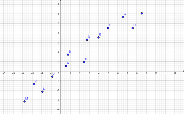
Figure 8-3. Scattered linear data
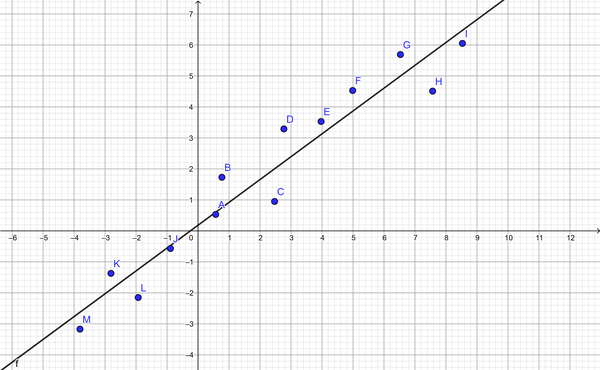
Figure 8-4. Predicted line of best fit using TensorFlow.js
Now that you’re familiar with the basics of training, you can expand your process to understanding what it takes to solve more complex models. Training a model is significantly dependent on the architecture and the quality and quantity of the data.
Nonlinear Training 101
If every problem were based on lines, there would be no need for machine learning. Statisticians have been solving linear regression since the early 1800s. Unfortunately, this fails as soon as your data is nonlinear. What would happen if you asked the AI to solve for Y = X2?
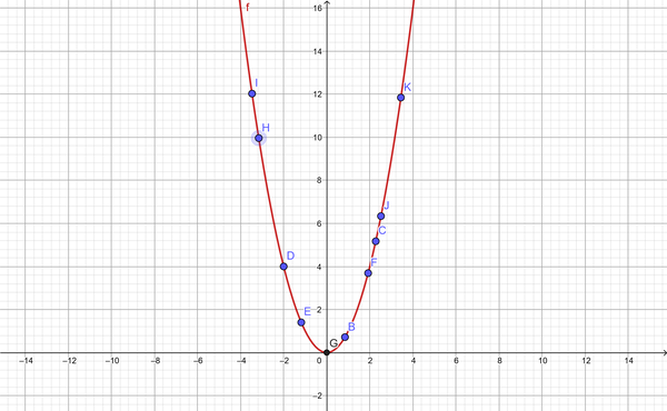
Figure 8-5. Simple Y = X2
More complex problems require more complex model architecture. In this section, you’ll learn new properties and features of a layers-based model, as well as tackle a nonlinear grouping of data.
You can add far more nodes to a neural network, but they would all still exist in a grouping of linear functions. To break linearity, it’s time to add activation functions.
Activation functions work similarly to neurons in the brain. Yes, this analogy again. When a neuron electrochemically receives a signal, it doesn’t always activate. There’s a threshold needed before a neuron fires its action potential. Similarly, neural networks have a degree of bias and similar on/off action potentials that occur when they reach their threshold due to incoming signals (similar to depolarizing current). Succinctly put, activation functions make neural networks capable of nonlinear predictions.2
Note
There are smarter ways to solve quadratic functions if you know that you want your solution to be quadratic. The way you will solve for X2 in this section is orchestrated explicitly for learning more about TensorFlow.js, rather than solving for simple mathematical functions.
Yes, this exercise could be solved easily without using AI, but what fun would that be?
Gathering the Data
Exponential functions can return some pretty large numbers, and one of the tricks to speed up model training is to keep numbers and their distance between each other small. You’ll see this time and time again. For our purposes, the training data for the model will be numbers between 0 and 10.
constjsxs=[];constjsys=[];constdataSize=10;conststepSize=0.001;for(leti=0;i<dataSize;i=i+stepSize){jsxs.push(i);jsys.push(i*i);}// Inputsconstxs=tf.tensor(jsxs);// Answers we want from inputsconstys=tf.tensor(jsys);
This code prepares two tensors. The xs tensor is a grouping of 10,000 values, and ys is the square of these.
Adding Activations to Neurons
Choosing your activation functions for the neurons in a given layer, and your model size, is a science in itself. It depends on your goals, your data, and your knowledge. Just like with code, you can come up with several solutions that all work nearly as well as another. It’s experience and practice that help you find solutions that fit.
When adding activation, it’s important to note there are quite a few activation functions built into TensorFlow.js. One of the most popular activation functions is called ReLU, which stands for Rectified Linear Unit. As you might have gathered from the name, it comes from the heart of scientific terminology rather than witty NPM package names. There is all kinds of literature on the benefits of using ReLU over various other activation functions for some models. You must know ReLU is a popular choice for an activation function, and you’re likely to be just fine starting with it. You should feel free to experiment with other activation functions as you learn more about model architecture. ReLU helps models train faster, compared to many alternatives.
In the last model, you had only a single node and an output. Now it’s important to grow the size of the network. There’s no formula for what size to use, so the first phase of each problem usually takes a bit of experimenting. For our purposes, we’ll increase the model with one dense layer of 20 neurons. A dense layer means that every node in that layer is connected to each node in the layers before and after it. The resulting model looks like Figure 8-6.

Figure 8-6. Neural network architecture (20 neurons)
To tour the architecture displayed in Figure 8-6 from left to right, one number enters the network, the 20-neuron layer is called a hidden layer, and the resulting value is output in the final layer. Hidden layers are the layers between the input and output. These hidden layers add trainable neurons and make the model able to process more complex patterns.
To add this layer and provide it with an activation function, you’ll specify a new dense layer in the sequence:
model.add(tf.layers.dense({inputShape:1,units:20,activation:"relu"}));model.add(tf.layers.dense({units:1}));
The first layer defines the input tensor as a single number.
Specify the layer should be 20 nodes.
Specify a fancy activation function for your layer.
Add the final single-unit layer for the output value.
If you compile the model and print the summary, you’ll see output similar to Example 8-3.
Example 8-3. Calling model.summary() for the current structure
_________________________________________________________________
Layer (type)                 Output shape              Param #
=================================================================
dense_Dense1 (Dense)         [null,20]                 40
_________________________________________________________________
dense_Dense2 (Dense)         [null,1]                  21
=================================================================
Total params: 61
Trainable params: 61
Non-trainable params: 0
_________________________________________________________________
This model architecture has two layers that match the previous layer-creation code. The null sections represent the batch size, and since that can be any number, it is left blank. For example, the first layer is represented as [null,20], so a batch of four values would give the model the input of [4, 20].
You’ll notice the model has a total of 61 tunable parameters. If you review the diagram in Figure 8-6, you can do the lines and nodes to get the parameters. The first layer has 20 nodes and 20 lines to them, which is why it has 40 parameters. The second layer has 20 lines all going to a single node, which is why that has only 21 parameters. Your model is ready to train, but it’s significantly bigger this time.
If you make these changes and kick off training, you’ll likely hear your CPU/GPU fan spin up and see a bunch of nothing. It sounds like the computer might be training, but it sure would be nice to see some kind of progress.
Watching Training
TensorFlow.js has all kinds of amazing tools for helping you identify progress on training. Most particularly, there is a property of the fit configuration called callbacks. Inside the callbacks object, you can tie in with certain life cycles of the training model and run whatever code you’d like.
As you’re already familiar with an epoch (one full run through the training data), that’s the moment you’ll use in this example. Here’s a terse but effective method for getting some kind of console messaging.
constprintCallback={onEpochEnd:(epoch,log)=>{console.log(epoch,log);}};
Create the callback object that contains all the life cycle methods you’d like to tie into.
onEpochEndis one of the many identified life cycle callbacks that training supports. The others are enumerated in thefitsection of the framework documentation.Print the values for review. Normally, you would do something more involved with this information.
Note
An epoch can be redefined by setting the stepsPerEpoch number in the fit config. Using this variable, an epoch can become any number of training data. By default, this is set to null, and therefore an epoch is set to the quantity of unique samples in your training set divided by the batch size.
All that’s left to do is pass your object to the model’s fit configuration alongside your epochs, and you should see logs while your model is training.
awaitmodel.fit(xs,ys,{epochs:100,callbacks:printCallback});
The onEpochEnd callbacks print to your console, showing that the training is working. In Figure 8-7, you can see your epoch and your log object.
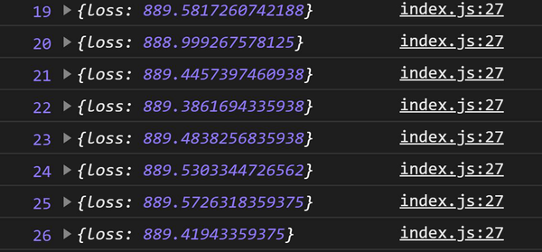
Figure 8-7. The onEpochEnd log for epochs 19 through 26
It’s a breath of fresh air to be able to see the model is actually training and to even tell what epoch it’s on. But, what’s going on with the log values?
Model logs
A model is told how to define loss with a loss function. What you want to see in each epoch is that the loss goes down. The loss is not only “is this right or wrong?” It’s about how wrong the model was so that it can learn. After each epoch, the model is reporting the loss, and in a good model architecture, this number goes down quickly.
You’re probably interested in seeing the accuracy. Most of the time, accuracy is a great metric, and we could enable accuracy in the logs. However, for a model like this, accuracy isn’t a very good fit as a metric. For instance, if you asked the model what the predicted output for [7] should be and the model answers 49.0676842 instead of 49, its accuracy is zero because it was incorrect. While the close result would have a low loss and would be accurate after rounding, it’s technically wrong, and the
accuracy score of the model would be poor. Let’s enable accuracy later when it works more effectively.
Improving Training
The loss values are pretty high. What is a high loss value? Concretely, it depends on the problem. However, when you see 800+ in error values, it’s generally safe to say it’s not done training.
Adam optimizer
Fortunately, you don’t have to leave your computer training for weeks. Currently, the optimizer is set to the defaults of stochastic gradient descent (sgd). You can modify the sgd presets or even choose a different optimizer. One of the most popular optimizers is called Adam. If you’re interested in trying Adam, you don’t have to read the paper on Adam published in 2015; you simply need to change the value of sgd to adam, and now you’re good to go. This is where you can enjoy the benefit of a framework. Simply by changing a small string, your entire model architecture has changed. Adam has significant benefits for solving certain types of problems.
The updated compile code looks like this:
model.compile({optimizer:"adam",loss:"meanSquaredError"});
With the new optimizer, the loss drops below 800 within a few epochs, and it even drops below one, as you can see in Figure 8-8.

Figure 8-8. The onEpochEnd log for epochs 19 through 26
After 100 epochs, the model was still making progress for me but stopped at a loss value of 0.03833026438951492. This varies on each run, but as long as the loss is small, the model will work.
Tip
The practice of modifying and adjusting the model architecture to train or converge faster for a particular problem is a mix of experience and experiments.
Things are looking good, but there’s one more feature we should add that sometimes cuts training time down significantly. On a pretty decent machine, these 100 epochs take around 100 seconds to run. You can speed up your training by batching data with a single line. When you assign the batchSize property to the fit configuration, training gets substantially faster. Try adding a batch size to your fit call:
awaitmodel.fit(xs,ys,{epochs:100,callbacks:printCallback,batchSize:64});
This
batchSizeof 64 cut training from 100 seconds to 50 for my machine.
Note
Batch sizes are trade-offs of efficiency for memory. If the batch is too large, this will limit which machines are capable of running the training.
You have a model that trains within a reasonable time for next to no cost on size. However, increasing the batch size is an option you can and should review.
More nodes and layers
This whole time the model has been the same shape and size: one “hidden” layer of 20 nodes. Don’t forget, you can always add more layers. As an experiment, add another layer of 20 nodes, so your model architecture looks like Figure 8-9.

Figure 8-9. Neural network architecture (20 × 20 hidden nodes)
With the Layers model architecture, you can build this model by adding a new layer. See the following code:
model.add(tf.layers.dense({inputShape:1,units:20,activation:"relu"}));model.add(tf.layers.dense({units:20,activation:"relu"}));model.add(tf.layers.dense({units:1}));
The resulting model trains slower, which makes sense, but also converges faster, which also makes sense. This bigger model generates the correct value for the input [7] with only 30 epochs in a training time of 20 seconds.
Putting it all together, your resulting code does the following:
-
Creates several deeply connected layers that utilize ReLU activation
-
Sets the model to use advanced Adam optimization
-
Trains the model using the data in 64-chunk batches and prints progress along the way
The entire source code from start to finish looks like this:
constjsxs=[];((("improving training","adding more neurons and layers")))constjsys=[];// Create the datasetconstdataSize=10;conststepSize=0.001;for(leti=0;i<dataSize;i=i+stepSize){jsxs.push(i);jsys.push(i*i);}// Inputsconstxs=tf.tensor(jsxs);// Answers we want from inputsconstys=tf.tensor(jsys);// Print the progress on each epochconstprintCallback={onEpochEnd:(epoch,log)=>{console.log(epoch,log);}};// Create the modelconstmodel=tf.sequential();model.add(tf.layers.dense({inputShape:1,units:20,activation:"relu"}));model.add(tf.layers.dense({units:20,activation:"relu"}));model.add(tf.layers.dense({units:1}));// Compile for trainingmodel.compile({optimizer:"adam",loss:"meanSquaredError"});// Train and print timingconsole.time("Training");awaitmodel.fit(xs,ys,{epochs:30,callbacks:printCallback,batchSize:64});console.timeEnd("Training");// evaluate the modelconstnext=tf.tensor([7]);constanswer=model.predict(next);answer.();// Cleanup!answer.dispose();xs.dispose();ys.dispose();model.dispose();
The printed result tensor is exceptionally close to 49. The training works. While this has been a bit of a strange adventure, it highlighted part of the model creation and validation process. Building models is one of the skills you’ll acquire over time as you experiment with various data and its associated solutions.
In subsequent chapters, you’ll solve more elaborate but rewarding problems, like classification. Everything you’ve learned here will be a tool in your workbench.
Chapter Review
You’ve entered the world of training models. The layer model structure is not only an understandable visual, but now it’s something you can comprehend and build on demand. Machine learning is very different from normal software development, but you’re on your way to comprehending the differences and benefits afforded by TensorFlow.js.
Chapter Challenge: The Model Architect
Now it’s your turn to build a Layers model via specification. What does this model do? No one knows! It’s not going to be trained with any data at all. In this challenge, you’ll be tasked to build a model with all kinds of properties you might not understand, but you should be familiar enough to at least set up the model. This model will be the biggest you’ve created yet. Your model will have five inputs and four outputs with two layers between them. It will look like Figure 8-10.
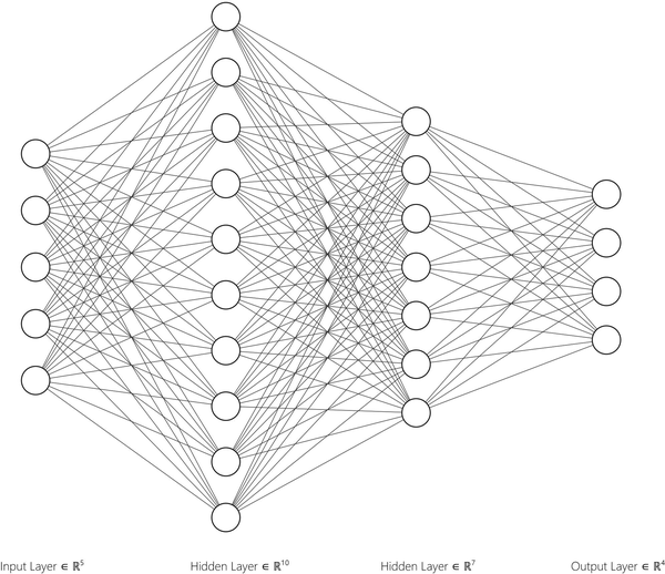
Figure 8-10. The Chapter Challenge model
Do the following in your model:
-
The input layer should have 5 units.
-
The next layer should have 10 units and use sigmoid for activation.
-
The next layer should have 7 units and use ReLU activation.
-
The final layer should have 4 units and use softmax for activation.
-
The model should use Adam optimization.
-
The model should use the loss function
categoricalCrossentropy.
Before building this model and looking at the summary, can you calculate how many trainable parameters the final model will have? That’s the total number of lines and circles from Figure 8-10, not counting the input.
You can find the answer to this challenge in Appendix B.
Review Questions
Let’s review the lessons you’ve learned from the code you’ve written in this chapter. Take a moment to answer the following questions:
-
Why would the Chapter Challenge model not work with the training data from this chapter?
-
What method can you call on a model to log and review its structure?
-
Why do you add activation functions to layers?
-
How do you specify the input shape for the Layers model?
-
What does
sgdstand for? -
What is an epoch?
-
If a model has one input, then a layer of two nodes, and an output of two nodes, how many hidden layers are present?
Solutions to these exercises are available in Appendix A.
1 Supported optimizers are listed in tfjs-core’s optimizers folder.
2 Learn more about activation functions from Andrew Ng.