6

Non-Fragile Dynamic Output Feedback Control with Interval-Bounded Coefficient Variations

6.1    Introduction

In Chapters 2 and 3, the non-fragile state feedback and dynamic output feedback control problems with norm-bounded uncertainties are studied, respectively. However, this kind of uncertainty cannot exactly describe the uncertain information due to the finite word length (FWL) effects. Correspondingly, the interval type of parameter uncertainty [89] can describe the uncertain information more exactly than the former type. But in the design process, due to the fact that the vertices of the set of interval uncertain parameters grow exponentially with the number of uncertain parameters, which may result in numerical problems in computation for systems with high dimensions. Moreover, similar to the case in which the problem of designing a globally optimal full-order output-feedback controller for polytopic uncertain systems is known to be a non-convex NP-hard optimization problem [76], the problem of designing full-order non-fragile dynamic output feedback H_∞ controllers with an interval type of gain uncertainty is also a non-convex NP-hard one.

The purpose of this chapter is to design the controller which is assumed to be with additive gain variations of the interval type. And the full parameterized and sparse structured controllers are considered, respectively. For the full parameterized controller design problem, a two-step procedure is adopted to solve this non-convex problem. In Step 1, we give a design method of an initial controller gain C_k. In Step 2, with the controller gain C_k designed in Step 1, a linear matrix inequality (LMI)-based sufficient condition is given for the solvability of the non-fragile H_∞ control problem, which requires checking all of the vertices of the set of uncertain parameters that grows exponentially with the number of uncertain parameters. It will be very difficult to apply the result to systems with high dimensions. To overcome the difficulty, a notion of a structured vertex separator is proposed to approach the problem, and is exploited to develop sufficient conditions for the non-fragile H_∞ controller design in terms of solutions to a set of LMIs. The structured vertex separator method can significantly reduce the number of LMI constraints involved in the design conditions. For the sparse structured controller design problem, first, a class of sparse structures is specified from a given controller, which renders the resulting closed-loop system to be asymptotically stable and meet an H_∞ performance requirement, but it is fully parameterized. Then, a three-step procedure for non-fragile H_∞ controller design under the restriction of the sparse structure is provided. The contribution of this method is that it not only reduces the number of nontrivial parameters but also designs the sparse structured controllers with non-fragility. The resulting designs of the two cases guarantee that the closed-loop system is asymptotically stable and the H_∞ performance from the disturbance to the regulated output is less than a prescribed level.

6.2    Non-Fragile H_∞ Controller Design for Discrete-Time Systems

In this section, a two-step procedure is presented for solving the non-fragile H_∞ control problem, and a comparison is made between the new proposed method and the existing method.

6.2.1    Problem Statement

Consider a linear time-invariant (LTI) discrete-time system described by

$\begin{array}{ll}x\left(k+1\right)\hfill & =Ax\left(k\right)+B_1\omega \left(k\right)+B_{2}u\left(k\right)\hfill \\ z\left(k\right)\hfill & =C_{1}x\left(k\right)+D_{12}u\left(k\right)\hfill \\ y\left(k\right)\hfill & =C_{2}x\left(k\right)+D_{21}\omega \left(k\right)\hfill \end{array}$

(6.1)

where x(k) ∈ Rⁿ is the state, u(k) ∈ R^q is the control input, ω(k) ∈ R^r is the disturbance input, y(k) ∈ R^p is the measured output, and z(k) ∈ R^m is the regulated output, respectively, and A, B₁, B₂, C₁, C₂, D₁₂, and D₂₁ are known constant matrices of appropriate dimensions.

To formulate the control problem, we consider a controller with gain variations of the following form:

$\begin{array}{cc}\xi \left(k+1\right)& =\left(A_k+\text{Δ}{A}_k\right)\xi \left(k\right)+\left(B_k+\text{Δ}{B}_k\right)y\left(k\right)\\ u\left(k\right)& =\left(C_k+\text{Δ}{C}_k\right)\xi \left(k\right).\end{array}$

(6.2)

where ξ(k) ∈ Rⁿ is the controller state, and A_k, B_k, and C_k are controller gain matrices of appropriate dimensions to be designed. ΔA_k, ΔB_k, and ΔC_k represent the additive gain variations of the following interval types:

$\begin{array}{ll}\text{Δ}{A}_k\hfill & ={\left[{\theta }_{aij}\right]}_{n\times n},\left|{\theta }_{aij}\right|\le {\theta }_a,i,j=1,\cdots ,n,\hfill \\ \text{Δ}{B}_k\hfill & ={\left[{\theta }_{bij}\right]}_{n\times p},\left|{\theta }_{bij}\right|\le {\theta }_a,i=1,\cdots ,n,j=1,\cdots ,p,\hfill \\ \text{Δ}{C}_k\hfill & ={\left[{\theta }_{cij}\right]}_{q\times n},\left|{\theta }_{cij}\right|\le {\theta }_a,i=1,\cdots ,q,j=1,\cdots ,n.\hfill \end{array}$

(6.3)

Remark 6.1 The additive gain variations model of form (6.3) is from Li [89], which has been extensively used to describe the FWL effects.

Let e_k ∈ Rⁿ, h_k ∈ R^p, and g_k ∈ R^q denote the column vectors in which the kth element equals one and the others equal zero. Then the gain variations of the form (6.3) can be described as:

$\begin{array}{c}\text{Δ}{A}_k={\displaystyle \sum _{i=1}^n{\displaystyle \sum _{j=1}^n{\theta }_{aij}{e}_i{e}_j^T}},\text{Δ}{B}_k={\displaystyle \sum _{i=1}^n{\displaystyle \sum _{j=1}^p{\theta }_{bij}{e}_i{h}_j^T}},\\ \text{Δ}{C}_k={\displaystyle \sum _{i=1}^q{\displaystyle \sum _{j=1}^n{\theta }_{cij}{g}_i{e}_j^T}}.\end{array}$

Applying controller (6.2) to system (6.1), this yields the closed-loop system:

$\begin{array}{lll}{x}_e\left(k+1\right)\hfill & =\hfill & A_e{x}_e\left(k\right)+B_e\omega \left(k\right)\hfill \\ z\left(k\right)\hfill & =\hfill & C_e{x}_e\left(k\right)\hfill \end{array}$

(6.4)

where $x_e\left(k\right)={\left[\begin{array}{cc}x{\left(k\right)}^T& \text{ξ}{\left(k\right)}^t\end{array}\right]}^T$, and

$\begin{array}{c}{A}_e=\left[\begin{array}{cc}A& B_2\left(C_k+\text{Δ}{C}_k\right)\\ \left(B_k+\text{Δ}{B}_k\right)C_2& A_k+\text{Δ}{A}_k\end{array}\right],\\ B_e=\left[\begin{array}{c}{B}_1\\ B_k+\text{Δ}{B}_k{D}_{21}\end{array}\right],C_e=\left[\begin{array}{ll}{C}_1\hfill & D_{12}\left(C_k+\text{Δ}{C}_k\right)\hfill \end{array}\right].\end{array}$

Denote the transfer function from the disturbance ω to the controlled output z, corresponding to the state-space model (6.4), as

$G_{z\omega }\left(z\right)=C_e{\left(zI-A_e\right)}^{-1}{B}_e.$

This chapter addresses the following problem.

Non-fragile H_∞ control problem with controller gain variations: Given a positive constant γ, find a dynamic output feedback controller of the form (6.2) with the gain variations (6.3) such that the resulting closed-loop system (6.4) is asymptotically stable and ‖G_zω(z)‖ < γ.

6.2.2    Non-Fragile H_∞ Controller Design Methods

In this section, the non-fragile H_∞ controller design method will be given by two steps. First, we will give the design method of the controller gain C_k. Then, with the designed controller gain C_k, the non-fragile H_∞ controller design method is presented.

In the following, we focus on the problem of finding an initial feasible solution C_k to the non-fragile H_∞ control problem.

Consider controller (6.2) with ΔA_k = 0 and ΔB_k = 0, which is described by

$\begin{array}{lll}\dot{\xi }\left(k\right)\hfill & =\hfill & A_k\xi \left(k\right)+B_{k}y\left(k\right),\hfill \\ u\left(k\right)\hfill & =\hfill & \left(C_k+\text{Δ}{C}_k\right)\xi \left(k\right)\hfill \end{array}$

(6.5)

where ΔC_k is considered with the following norm-bounded form:

$\text{Δ}{C}_k=M_c{F}_3\left(t\right)E_c,$

where

$\begin{array}{l}{M}_c=\left[M_{c1}\cdots M_{cnq}\right],E_c={\left[E_{c1}^T\cdots E_{cnq}^T\right]}^T\hfill \\ M_{ck}=g_i,E_{ck}=e_j^T\hfill \\ k=n^2+np+\left(i-1\right)n+j,i=1,\cdots ,q, j=1,\cdots ,n\hfill \end{array}$

and $F_3^T\left(t\right)F_3\left(t\right)\le {\theta }_a^{2}I$ represent the uncertain parameters. Here θ_a is the same as before.

Combining controller (6.5) with system (6.1), we obtain the following closed-loop system:

$\begin{array}{lll}{\dot{x}}_e\left(k\right)\hfill & =\hfill & A_{edc}{x}_e\left(k\right)+B_{edc}\omega \left(k\right),\hfill \\ z\left(k\right)\hfill & =\hfill & C_e{x}_e\left(k\right),\hfill \end{array}$

(6.6)

where

$A_{edc}=\left[\begin{array}{cc}A& B_2\left(C_k+\text{Δ}{C}_k\right)\\ B_k{C}_2& A_k\end{array}\right],B_{edc}=\left[\begin{array}{c}{B}_1\\ B_k{D}_{21}\end{array}\right],$

and C_e is the same as the one in (6.4).

Then the following theorem gives a design method of the initial controller gain C_k.

Theorem 6.1 Consider system (6.1), where γ > 0 and θ_a > 0 are constants. If there exist matrices $\widehat{A},\widehat{B},\widehat{C},X>0,Y>0$, and a constant ε_c > 0 such that the following LMI holds:

$\begin{array}{c}[\begin{array}{lllll}-X\hfill & -I\hfill & 0\hfill & AX+B_2\widehat{C}\hfill & A\hfill \\ \ast \hfill & -Y\hfill & 0\hfill & \widehat{A}\hfill & YA+\widehat{B}{C}_2\hfill \\ \ast \hfill & \ast \hfill & -I\hfill & C_{1}X+D_{12}\widehat{C}\hfill & C_1\hfill \\ \ast \hfill & \ast \hfill & \ast \hfill & -X\hfill & -I\hfill \\ \ast \hfill & \ast \hfill & \ast \hfill & \ast \hfill & -Y\hfill \\ \ast \hfill & \ast \hfill & \ast \hfill & \ast \hfill & \ast \hfill \\ \ast \hfill & \ast \hfill & \ast \hfill & \ast \hfill & \ast \hfill \\ \ast \hfill & \ast \hfill & \ast \hfill & \ast \hfill & \ast \hfill \end{array}\\ \begin{array}{lll}{B}_1\hfill & B_2{M}_c\hfill & 0\hfill \\ Y{B}_1+\widehat{B}{D}_{21}\hfill & Y{B}_2{M}_c\hfill & 0\hfill \\ 0\hfill & D_{12}{M}_c\hfill & 0\hfill \\ 0\hfill & 0\hfill & {\epsilon }_c{\theta }_{a}X{E}_c^T\hfill \\ 0\hfill & 0\hfill & 0\hfill \\ -{\gamma }^{2}I\hfill & 0\hfill & 0\hfill \\ \ast \hfill & -{\epsilon }_{c}I\hfill & 0\hfill \\ \ast \hfill & \ast \hfill & -{\epsilon }_{c}I\hfill \end{array}]<0,\end{array}$

(6.7)

then controller (6.5) with

$\begin{array}{l}{A}_k={\left(X^{-1}-Y\right)}^{-1}\left(\widehat{A}-YAX-\widehat{B}{C}_{2}X-Y{B}_2\widehat{C}\right)X^{-1},\\ B_k={\left(X^{-1}-Y\right)}^{-1}\widehat{B},C_k=\widehat{C}{X}^{-1}\end{array}$

(6.8)

solves the non-fragile H_∞ control problem for system (6.1).

Proof 6.1 By Lemma 2.5, it is sufficient to shew that there exists a symmetric matrix P > 0 with the structure (2.11), such that

$\left[\begin{array}{cccc}-P& 0& P{A}_{edc}& P{B}_{edc}\\ \ast & -I& C_e& 0\\ \ast & \ast & -P& 0\\ \ast & \ast & \ast & -{\gamma }^{2}I\end{array}\right]<0.$

(6.9)

Equation (6.9) can be further written as

${\overline{Q}}_s+\text{Δ}{M}_{10}+\text{Δ}{M}_{10}^T<0,$

(6.10)

where

$\begin{array}{l}{\overline{Q}}_s=\left[\begin{array}{cccc}-P& 0& P{A}_{e0}& P{B}_{e0}\\ \ast & -I& C_{e0}& 0\\ \ast & \ast & -P& 0\\ \ast & \ast & \ast & -{\gamma }^{2}I\end{array}\right],\\ \text{Δ}{M}_{10}=\left[\begin{array}{cccc}0& 0& P\left[\begin{array}{cc}0& B_2\text{Δ}{C}_k\\ 0& 0\end{array}\right]& 0\\ 0& 0& \left[\begin{array}{cc}0& D_{12}\text{Δ}{C}_k\end{array}\right]& 0\\ 0& 0& 0& 0\\ 0& 0& 0& 0\end{array}\right].\end{array}$

It is easy to see that

$\text{Δ}{M}_{10}+\text{Δ}{M}_{10}^T={\text{Σ}}_1{F}_3\left(t\right){\text{Σ}}_2+{\left({\text{Σ}}_1{F}_3\left(t\right){\text{Σ}}_2\right)}^T,$

(6.11)

where ${\text{Σ}}_1=\left[\begin{array}{c}P\left[\begin{array}{c}{B}_2{M}_c\\ 0\end{array}\right]\\ D_{12}{M}_c\\ 0\\ 0\end{array}\right],{\text{Σ}}_2=\left[\begin{array}{cccc}0& 0& \left[\begin{array}{cc}0& E_c\end{array}\right]& 0\end{array}\right].$

By Lemma 2.12, for any positive scalar ε_c, (6.10) holds if and only if the following inequality holds:

${\overline{Q}}_s+\frac{1}{{\epsilon }_c}{\text{Σ}}_1{\text{Σ}}_1^T+{\epsilon }_c{\theta }_a^2{\text{Σ}}_2^T{\text{Σ}}_2\le 0.$

(6.12)

By the Schur complement, (6.10) is equivalent to

$\left[\begin{array}{ccc}{\overline{Q}}_s& {\text{Σ}}_1& {\epsilon }_c{\theta }_a{\text{Σ}}_2^T\\ \ast & -{\epsilon }_{c}I& 0\\ \ast & \ast & -{\epsilon }_{c}I\end{array}\right]<0.$

(6.13)

As in Scherer, Gahinet, and Chilali [113], partition P^–1 as

$P^{-1}=\left[\begin{array}{cc}X& M\\ M^T& \ast \end{array}\right].$

(6.14)

Due to the fact that P is with structure (2.11), it is easy to obtain X = M and X^–1 = Y + N.

Similar to the method in Scherer, Gahinet, and Chilali [113], let ${\text{Γ}}_1=\left[\begin{array}{cc}X& 1\\ X& 0\end{array}\right]$ Denote $\overline{\text{Γ}}=diag\left\{{\text{Γ}}_1,I,I,I,I\right\}$,perform a congruence transformation with $\overline{\text{Γ}}$ on (6.13) and with gain matrices (6.8), (6.13) is equivalent to (6.7). Thus, the proof is complete.

Remark 6.2 Theorem 6.1 shows that the non-fragile controller design problem with ΔA_k = 0, ΔB_k = 0, and ΔC_k with the norm-bounded uncertainty can be converted into a convex one depending on a single parameter ε_c > 0.

Then, with the designed C_k we will give the non-fragile H_∞ dynamic output feedback controller design method in the following.

To facilitate the presentation, we denote

$M_0\left(\text{Δ}{A}_k,\text{Δ}{B}_k,\text{Δ}{C}_k\right)=\left[\begin{array}{cccccc}{\text{Ξ}}_1& {\text{Ξ}}_2& 0& {\text{Ξ}}_4& S^{T}A& S^T{B}_1\\ \ast & {\text{Ξ}}_3& 0& {\text{Ξ}}_5& {\text{Ξ}}_6& {\text{Ξ}}_7\\ \ast & \ast & -I& {\text{Ξ}}_8& C_1& 0\\ \ast & \ast & \ast & -{\overline{P}}_{11}& -{\overline{P}}_{12}& 0\\ \ast & \ast & \ast & \ast & -{\overline{P}}_{22}& 0\\ \ast & \ast & \ast & \ast & \ast & -{\gamma }^{2}I\end{array}\right]$

(6.15)

where

$\begin{array}{l}{\text{Ξ}}_1={\overline{P}}_{11}-S-S^T,{\text{Ξ}}_2={\overline{P}}_{12}-S-S^T,\hfill \\ {\text{Ξ}}_3={\overline{P}}_{22}-S-S^T+N+N^T,\hfill \\ {\text{Ξ}}_4=S^{T}A+S^T{B}_2\left(C_k+\text{Δ}{C}_k\right)\hfill \\ {\text{Ξ}}_5={\left(S-N\right)}^{T}A+F_B{C}_2+N^T\text{Δ}{B}_k{C}_2+F_A\hfill \\ +N^T\text{Δ}{A}_k+{\left(S-N\right)}^T{B}_2\left(C_k+\text{Δ}{C}_k\right),\hfill \\ {\text{Ξ}}_6={\left(S-N\right)}^{T}A+F_B{C}_2+N^T\text{Δ}{B}_k{C}_2,\hfill \\ {\text{Ξ}}_7={\left(S-N\right)}^T{B}_1+F_B{D}_{21}+N^T\text{Δ}{B}_k{D}_{21},\hfill \\ {\text{Ξ}}_8=C_1+D_{12}\left(C_k+\text{Δ}{C}_k\right).\hfill \end{array}$

(6.16)

Then the following theorem presents a sufficient condition for the solvability of the non-fragile H_∞ control problem with additive uncertainty.

Theorem 6.2 Consider system (6.1). Let scalars γ > 0, θ_a > 0 and gain matrix C_k be given. If there exist matrices F_A, F_B, S, N, ${\overline{P}}_{12}$, and ${\overline{P}}_{11}>0,{\overline{P}}_{22}>0$, such that the following LMIs hold:

$\begin{array}{c}{M}_0\left(\text{Δ}{A}_k,\text{Δ}{B}_k,\text{Δ}{C}_k\right)<0,{\theta }_{aij},{\theta }_{bik},{\theta }_{clj}\in \left\{-{\theta }_a,{\theta }_a\right\},\\ i,j=1,\mathrm{...},n;k=1,\mathrm{...},p;l=1,\mathrm{...},q,\end{array}$

(6.17)

then controller (6.2) with additive uncertainty described by (6.3), C_k, and

$A_k={\left(N^T\right)}^{-1}{F}_A,B_k={\left(N^T\right)}^{-1}{F}_B,$

(6.18)

solves the non-fragile H_∞ control problem for system (6.1).

Proof 6.2 By Lemma 2.5, it is sufficient to show that there exist a matrix G with structure (2.14) and a symmetric positive matrix $P=\left[\begin{array}{cc}{P}_{11}& P_{12}\\ P_{12}^T& P_{22}\end{array}\right]>0$ such that

$M_1=\left[\begin{array}{cccc}P-G-G^T& 0& G^T{A}_e& G^T{B}_e\\ \ast & -I& C_e& 0\\ \ast & \ast & -P& 0\\ \ast & \ast & \ast & -{\gamma }^{2}I\end{array}\right]<0$

(6.19)

holds for all θ_aij, θ_bik, and θ_clj satisfying (6.3).

Denote

$\begin{array}{l}S=Y+N,{\text{Γ}}_1=\left[\begin{array}{cc}I& I\\ I& 0\end{array}\right],{\overline{\text{Γ}}}_1=diag\left\{{\text{Γ}}_1,I,{\text{Γ}}_1,I\right\},\\ {\overline{P}}_{11}=P_{11}+P_{12}+P_{12}^T+P_{22},{\overline{P}}_{12}=P_{11}+P_{12}^T,{\overline{P}}_{22}=P_{11}.\end{array}$

Then (6.19) is equivalent to

$\begin{array}{lll}{M}_2\hfill & =\hfill & {\overline{\text{Γ}}}_1{M}_1{\overline{\text{Γ}}}_1^T\hfill \\ \hfill & =\hfill & \left[\begin{array}{cccccc}{\text{Ξ}}_1& {\text{Ξ}}_2& 0& {\text{Ξ}}_4& S^{T}A& S^T{B}_1\\ \ast & {\text{Ξ}}_3& 0& {\Pi }_1& {\Pi }_2& {\Pi }_3\\ \ast & \ast & -I& {\text{Ξ}}_8& C_1& 0\\ \ast & \ast & \ast & -{\overline{P}}_{11}& -{\overline{P}}_{12}& 0\\ \ast & \ast & \ast & \ast & -{\overline{P}}_{22}& 0\\ \ast & \ast & \ast & \ast & \ast & -{\gamma }^{2}I\end{array}\right]<0\hfill \end{array}$

(6.20)

which holds for all θ_aij, θ_bik, and θ_cij satisfying (6.3), where ${\text{Ξ}}_1,{\text{Ξ}}_2,{\text{Ξ}}_3,{\text{Ξ}}_4$ are defined by (6.16), and

$\begin{array}{lll}{\Pi }_1\hfill & =\hfill & {\left(S-N\right)}^{T}A+N^T{B}_k{C}_2+N^T\text{Δ}{B}_k{C}_2+N^T{A}_k+N^T{A}_k+{\left(S-N\right)}^T{B}_2\left(C_k+\text{Δ}{C}_k\right),\hfill \\ {\Pi }_2\hfill & =\hfill & {\left(S-N\right)}^{T}A+N^T{B}_k{C}_2+N^T\text{Δ}{B}_k{C}_2,\hfill \\ {\Pi }_3\hfill & =\hfill & {\left(S-N\right)}^T{B}_1+N^T{B}_k{D}_{21}+N^T\text{Δ}{B}_k{C}_{21}.\hfill \end{array}$

By (6.18), (6.19), and the Schur complement, it concludes that (6.20) is equivalent to (6.17).

Thus, the proof is complete.

Remark 6.3 Theorem 6.2 presents a sufficient condition in terms of solutions to a set of LMIs for the solvability of the non-fragile H_∞ control problem. By the proofs of Theorem 6.2 and Lemma 2.5, Theorem 6.2 also shows that the non-fragile H_∞ control problem becomes a convex one when the gain matrix C_k is known and the state-space realizations of the designed controllers with gain variations admit the slack variable matrix G with the structure of (2.14).

However, for the non-fragile H_∞ controller design method, it should be noted that the number of LMIs involved in (6.17) is 2^n2+np+nq, which results in the difficulty of implementing the LMI constraints in computation. For example, when n = 6 and p = q = 1, the number of LMIs involved in (6.17) is 2⁴⁸, which already exceeds the capacity of the current LMI solver in MATLAB. To overcome the difficulty arising from implementing the design condition given in Theorem 6.2, the following method is developed.

Denote

$\begin{array}{lll}{F}_{a1}\hfill & =\hfill & \left[\begin{array}{llll}{f}_{a11}\hfill & f_{a12}\hfill & \cdots \hfill & f_{a1l_a}\hfill \end{array}\right],\hfill \\ F_{a2}\hfill & =\hfill & {\left[\begin{array}{llll}{f}_{a21}^T\hfill & f_{a22}^T\hfill & \cdots \hfill & f_{a1l_a}\hfill \end{array}\right]}^T\hfill \end{array}$

(6.21)

where l_a = n² + np + nq, and

$\begin{array}{lll}{f}_{a1k}\hfill & =\hfill & {\left[\begin{array}{llllll}{0}_{1\times n}\hfill & {\left(N^T{e}_i\right)}^T\hfill & 0_{1\times q}\hfill & 0_{1\times n}\hfill & 0_{1\times n}\hfill & 0_{1\times r}\hfill \end{array}\right]}^T,\hfill \\ f_{a2k}\hfill & =\hfill & \left[\begin{array}{llllll}{0}_{1\times n}\hfill & 0_{1\times n}\hfill & 0_{1\times q}\hfill & e_j^T\hfill & 0_{1\times n}\hfill & 0_{1\times r}\hfill \end{array}\right],\hfill \\ \text{for }k\hfill & =\hfill & \left(i-1\right)n+j,i,j=1,\mathrm{\cdots },n.\hfill \\ f_{a1k}\hfill & =\hfill & {\left[\begin{array}{llllll}{0}_{1\times n}\hfill & {\left(N^T{e}_i\right)}^T\hfill & 0_{1\times q}\hfill & 0_{1\times n}\hfill & 0_{1\times n}\hfill & 0_{1\times r}\hfill \end{array}\right]}^T,\hfill \\ f_{a2k}\hfill & =\hfill & \left[\begin{array}{llllll}{0}_{1\times n}\hfill & 0_{1\times n}\hfill & 0_{1\times q}\hfill & h_j^T{C}_2\hfill & h_j^T{C}_2\hfill & h_j^T{D}_{21}\hfill \end{array}\right],\hfill \\ \text{for }k\hfill & =\hfill & n^2+\left(i-1\right)p+j,i=1,\mathrm{\cdots },n,j=1,\mathrm{\cdots },p.\hfill \\ f_{a1k}\hfill & =\hfill & {\left[\begin{array}{llllll}{\left(S^T{B}_{2gi}\right)}^T\hfill & {\left({\left(S-N\right)}^T{B}_{2gi}\right)}^T\hfill & {\left(D_{12gi}\right)}^T\hfill & 0_{1\times n}\hfill & 0_{1\times n}\hfill & 0_{1\times r}\hfill \end{array}\right]}^T,\hfill \\ f_{a2k}\hfill & =\hfill & \left[\begin{array}{llllll}{0}_{1\times n}\hfill & 0_{1\times n}\hfill & 0_{1\times q}\hfill & e_j^T\hfill & 0_{1\times n}\hfill & 0_{1\times r}\hfill \end{array}\right],\hfill \\ \text{for }k\hfill & =\hfill & n^2+np+\left(i-1\right)n+j,i=1,\mathrm{\cdots },q,j=1,\mathrm{\cdots },n.\hfill \end{array}$

Let k₀, k₁, …, k_Sa be integers satisfying

$k_0=0<k_1<\mathrm{\cdots }<k_{s_a}=l_a$

and matrix Σ have the following structure:

$\text{Σ}=\left[\begin{array}{cc}diag\left[{\sigma }_{11}^1\cdots {\sigma }_{11}^{s_a}\right]& diag\left[{\sigma }_{12}^1\cdots {\sigma }_{12}^{s_a}\right]\\ diag{\left[{\sigma }_{12}^1\cdots {\sigma }_{12}^{s_a}\right]}^T& diag\left[{\sigma }_{22}^1\cdots {\sigma }_{22}^{s_a}\right]\end{array}\right],$

(6.22)

where ${\sigma }_{11}^i,{\sigma }_{12}^i,$ and ${\sigma }_{22}^i\in R^{\left(k_i-k_{i-1}\right)\times \left(k_i-k_{i-1}\right)},i=1,\cdots ,s_a$. Then, we have the following theorem.

Theorem 6.3 Consider system (6.1). Let scalars γ > 0, θ_a > 0, and gain matrix C_k be given. If there exist matrices F_A, F_B, S, N, ${\overline{P}}_{12}$, ${\overline{P}}_{11}>0$, ${\overline{P}}_{22}>0$, and symmetric matrix Σ with the structure described by (6.22) such that the following LMIs hold:

$\left[\begin{array}{cc}Q& F_{a1}\\ F_{a1}^T& 0\end{array}\right]+{\left[\begin{array}{cc}{F}_{a2}& 0\\ 0& I\end{array}\right]}^T\sum \left[\begin{array}{cc}{F}_{a2}& 0\\ 0& I\end{array}\right]<0,$

(6.23)

$\begin{array}{c}{\left[\begin{array}{c}I\\ diag\left[{\theta }_{k_{i-1}+j\cdots {\theta }_{k_i}}\right]\end{array}\right]}^T\left[\begin{array}{cc}{\sigma }_{11}^i& {\sigma }_{12}^i\\ {\left({\sigma }_{12}^i\right)}^T& {\sigma }_{22}^i\end{array}\right]\\ \times {\left[\begin{array}{c}I\\ diag\left[{\theta }_{k_{i-1}+j\cdots {\theta }_{k_i}}\right]\end{array}\right]}^T\ge 0,forall{\theta }_{k_{i-1}+j}\in \left\{-{\theta }_a,{\theta }_a\right\},\\ j=1,\cdots ,k_i-k_{i-1},i=1,\cdots ,s_a,\end{array}$

(6.24)

where

$Q=\left[\begin{array}{cccccc}{\text{Ξ}}_1& {\text{Ξ}}_2& 0& {\text{Ψ}}_1& S^{T}A& S^{T}B\\ \ast & {\text{Ξ}}_3& 0& {\text{Ψ}}_2& {\text{Ψ}}_3& {\text{Ψ}}_4\\ \ast & \ast & -I& C_1+D_{12}{C}_k& C_1& 0\\ \ast & \ast & \ast & -{\overline{P}}_{11}& -{\overline{P}}_{12}& 0\\ \ast & \ast & \ast & \ast & -{\overline{P}}_{22}& 0\\ \ast & \ast & \ast & \ast & \ast & -{\gamma }^{2}I\end{array}\right]$

(6.25)

with Ξ₁, Ξ₂, Ξ₃ defined by (6.16) and

$\begin{array}{lll}{\text{Ψ}}_1\hfill & =\hfill & S^{T}A+S^T{B}_2{C}_k\hfill \\ {\text{Ψ}}_2\hfill & =\hfill & {\left(S-N\right)}^{T}A+F_B{C}_2+F_A+{\left(S-N\right)}^T{B}_2{C}_k,\hfill \\ {\text{Ψ}}_3\hfill & =\hfill & {\left(S-N\right)}^{T}A+F_B{C}_2,\hfill \\ {\text{Ψ}}_4\hfill & =\hfill & {\left(S-N\right)}^T{B}_1+F_B{D}_{21},\hfill \end{array}$

then controller (6.2) with additive uncertainty described by (6.3) and the controller gain parameters given by (6.18) solve the non-fragile H_∞ control problem for system (6.1).

Proof 6.3 By (6.15), we have

$M_0=Q+\text{Δ}Q+\text{Δ}{Q}^T<0,$

(6.26)

where

$\text{Δ}Q=\left[\begin{array}{cccccc}0& 0& 0& \text{Δ}{Q}_1& 0& 0\\ 0& 0& 0& \text{Δ}{Q}_2& \text{Δ}{Q}_3& \text{Δ}{Q}_4\\ 0& 0& 0& \text{Δ}{Q}_5& 0& 0\\ 0& 0& 0& 0& 0& 0\\ 0& 0& 0& 0& 0& 0\\ 0& 0& 0& 0& 0& 0\end{array}\right]$

with

$\begin{array}{lll}\text{Δ}{Q}_1\hfill & =\hfill & S^T{B}_2{\displaystyle \sum _{i=1}^q{\displaystyle \sum _{j=1}^n{\theta }_{cij}{g}_i{e}_j^T,}}\hfill \\ \text{Δ}{Q}_2\hfill & =\hfill & {\displaystyle \sum _{i,j=1}^n{\theta }_{aij}{N}^T{e}_i{e}_j^T+{\displaystyle \sum _{i=1}^n{\displaystyle \sum _{j=1}^q{\theta }_{bij}{N}^T{e}_i{h}_j^T{C}_2+{\left(S-N\right)}^T{B}_2{\displaystyle \sum _{i=1}^q{\displaystyle \sum _{j=1}^n{\theta }_{cij}{g}_i{e}_j^T,}}}}}\hfill \\ \text{Δ}{Q}_3\hfill & =\hfill & {\displaystyle \sum _{i=1}^n{\displaystyle \sum _{j=1}^p{\theta }_{bij}{N}^T{e}_i{h}_j^T{C}_2,}}\hfill \\ \text{Δ}{Q}_4\hfill & =\hfill & {\displaystyle \sum _{i=1}^n{\displaystyle \sum _{j=1}^p{\theta }_{bij}{N}^T{e}_i{h}_j^T{D}_{21},}}\hfill \\ \text{Δ}{Q}_5\hfill & =\hfill & D_{12}{\displaystyle \sum _{i=1}^q{\displaystyle \sum _{j=1}^n{\theta }_{cij}{g}_j{e}_j^T.}}\hfill \end{array}$

By (6.21) and (6.26), it follows that (6.17) is equivalent to

$\begin{array}{lll}{M}_0\hfill & =\hfill & Q+{\displaystyle {\sum }_{i=1}^{la}{\theta }_i{f}_{a1i}{f}_{a2i}+{\left({\displaystyle {\sum }_{i=1}^{la}{\theta }_i{f}_{a1i}{f}_{a2i}}\right)}^T}\hfill \\ \hfill & =\hfill & Q+F_{a1}{\widetilde{\text{Δ}}}_a{F}_{a2}+{\left(F_{a1}{\widetilde{\text{Δ}}}_a{F}_{a2}\right)}^T<0\hfill \end{array}$

(6.27)

which holds for all |θ_i| ≤ θ_a, where ${\widetilde{\text{Δ}}}_a=diag\left[{\theta }_1,\cdots ,{\theta }_{la}\right]$. By Lemma 2.5, it follows that (6.27) holds if and only if there exists a symmetric matrix Σ ∈ R^{l_{a × la}} such that (6.23) and

${\left[\begin{array}{c}I\\ {\widetilde{\text{Δ}}}_a\end{array}\right]}^T\sum \left[\begin{array}{c}I\\ {\widetilde{\text{Δ}}}_a\end{array}\right]\ge 0$

(6.28)

hold for all θ_i ∈ {-θ_a, θ_a}, i = 1,…, l_a. Notice that the set of Σ satisfying (6.22) is a subset of the set of Σ satisfying (6.28), hence the conclusion follows.

Remark 6.4 From the proof of Theorem 6.3, it follows that when s_a = 1, the set of Σ satisfying (6.22) is equal to the set of Σ satisfying (6.28), and the design conditions given in Theorem 6.3 and Theorem 6.2 are equivalent. Σ satisfying (6.23) and (6.28) (or (6.24) with s_a = 1) is said to be a vertex separator [67]. Notice that the number of LMIs involved in (6.28) or (6.24) with s_a = 1 still is 2^{n2 + np + nq}, so that the difficulty of implementing the LMI constraints remains. To overcome the difficulty, Theorem 6.3 presents a sufficient condition for the non-fragile H_∞ controller design in terms of separator Σ with the structure described by (6.22), where the number of LMIs involved in (6.24) is ${\displaystyle {\sum }_{i=1}^{S_a}{2}^{k_i-k_{i-1}}},$, which can be controlled not to grow exponentially by reducing the value of max k_i–k_i–1 : i = 1,…, s_a. Compared with the Σ being of full block in (6.23) and (6.28), Σ with the structure described by (6.22) satisfying (6.23) and (6.24) is said to be a structured vertex separator. However, it should be noted that the design condition given in Theorem 6.3 may be more conservative than that given in Theorem 6.2 because of the structure constraint on Σ. But the smaller the value of s_a is, the less conservativeness is introduced.

To illustrate the comparison between the proposed method and the existing design method, the result of a non-fragile H_∞ controller design with norm-bounded gain variations is introduced in the following.

Similar to Yang, Wang, and Lin [149] and Mahmoud [103] for non-fragile problems with norm-bounded uncertainty, the norm-bounded type of gain variations ΔA_k, ΔB_k, and ΔC_k can be over-bounded [107] by the following norm-bounded uncertainty:

$\begin{array}{c}\text{Δ}{A}_k=M_a{F}_1\left(t\right)E_a,\text{Δ}{B}_k=M_b{F}_2\left(t\right)E_b,\\ \text{Δ}{C}_k=M_c{F}_3\left(t\right)E_c,\end{array}$

(6.29)

where

$\begin{array}{l}{M}_a=[M_{a1}\mathrm{\cdots }{M}_{a{n}^2}],E_a={[E_{a1}^T\mathrm{\cdots }{E}_{a{n}^2}^T]}^T,\hfill \\ M_b=[M_{b1}\mathrm{\cdots }{M}_{bnp}],E_b={[E_{b1}^T\mathrm{\cdots }{E}_{bnp}^T]}^T,\hfill \\ M_c=[M_{c1}\mathrm{\cdots }{M}_{cnq}],E_b={[E_{c1}^T\mathrm{\cdots }{E}_{cnq}^T]}^T,\hfill \end{array}$

with

$\begin{array}{l}{M}_{ak}=e_i,E_{ak}=e_j^T\\ \text{for }k=\left(i-1\right)n+j,i,j=1,\mathrm{\cdots },n,\\ M_{bk}=e_i,E_{bk}=h_j^T\\ \text{for }k=n^2+\left(i-1\right)p+j,i=1,\mathrm{\cdots },n,j=1,\mathrm{\cdots },p,\\ M_{ck}=g_i,E_{ck}=e_j^T\\ \text{for }k=n^2+np+\left(i-1\right)n+j,i=1,\mathrm{\cdots },q,j=1,\mathrm{\cdots },n\end{array}$

and $F_i^T\left(t\right)F_i\left(t\right)\le {\theta }_a^{2}I$ for i = 1, 2, 3, represent the uncertain parameters, here, θ_a is the same as before.

Noting that the problem of non-fragile dynamic output feedback H_∞controller design with norm-bounded gain variations is also a non-convex problem, and similar to Theorem 6.3, when the controller gain C_k is known, it can be converted to a convex one.

To facilitate the presentation, denote

${\overline{F}}_A=\overline{N}{A}_k,{\overline{F}}_B=\overline{N}{A}_B,$

$M_{a1}=\left[\begin{array}{ccc}0& \overline{S}{B}_2{M}_c& 0\\ \overline{N}{M}_a& \left(\overline{S}-\overline{N}\right)B_2{M}_c& \overline{N}{M}_b\\ 0& D_{12}{M}_c& 0\\ 0& 0& 0\\ 0& 0& 0\\ 0& 0& 0\end{array}\right],$

$M_{a2}=\left[\begin{array}{cccccc}0& 0& 0& E_a& 0& 0\\ 0& 0& 0& E_c& 0& 0\\ 0& 0& 0& E_b{C}_2& E_b{C}_2& E_b{D}_{21}\end{array}\right].$

Assume that C_k is known, by using the method in Yang, Wang, and Lin [149] and Mahmoud [103], the non-fragile H_∞ controller design with norm-bounded gain variations is reduced to solve the following LMI:

$\left[\begin{array}{ccc}\overline{Q}& M_{a1}& {\theta }_a\epsilon M_{a2}^T\\ \ast & -\epsilon I& 0\\ \ast & \ast & -\epsilon I\end{array}\right]<0,$

(6.30)

with matrix variables $\overline{S}>0,\overline{N}<0$, and scalar ε > 0, where

$\overline{Q}=\left[\begin{array}{cccccc}-\overline{S}& -\overline{S}& 0& \overline{S}\left(A+B_2{C}_k\right)& \overline{S}A& \overline{S}B\\ \ast & -\overline{S}+N& 0& Q_1& Q_2& Q_3\\ \ast & \ast & -I& C_1+D_{12}{C}_k& C_1& 0\\ \ast & \ast & \ast & -\overline{S}& -\overline{S}& 0\\ \ast & \ast & \ast & \ast & -\overline{S}+\overline{N}& 0\\ \ast & \ast & \ast & \ast & \ast & -{\gamma }^{2}I\end{array}\right],$

with

$\begin{array}{lll}{Q}_1\hfill & =\hfill & \left(\overline{S}-\overline{N}\right)\left(A+B_2{C}_k\right)+{\overline{F}}_A+F_B{C}_2,\hfill \\ Q_2\hfill & =\hfill & \left(\overline{S}-\overline{N}\right)A+{\overline{F}}_B{C}_2,\hfill \\ Q_3\hfill & =\hfill & \left(\overline{S}-\overline{N}\right)B_1+{\overline{F}}_B{D}_{21}.\hfill \end{array}$

The following lemma will show the relationship between condition (6.30) and the condition for designing non-fragile H_∞ controllers given in Theorem 6.3.

Lemma 6.1 Consider system (6.1). If condition (6.30) is feasible, then the condition for designing non-fragile H_∞ controllers given in Theorem 6.3 is feasible.

Proof 6.4 To proceed, let $\overline{S}={\overline{P}}_{11}={\overline{P}}_{12}=S,\overline{N}=N,\overline{S}-\overline{N}={\overline{P}}_{22}>0$. It is easy to see that $\overline{Q}=Q,M_{a1}=F_{a1,}$ and M_a2 = F_a2, that is, condition (6.30) becomes

$\left[\begin{array}{ccc}Q& F_{a1}& {\theta }_a\epsilon F_{a2}^T\\ \ast & -\epsilon I& 0\\ \ast & \ast & -\epsilon I\end{array}\right]<0.$

(6.31)

In Theorem 6.3, when s_a = l_a, according to (6.31) and $F_i^T\left(t\right)F_i\left(t\right)\le {\theta }_a^{2}I$, i = 1, 2, 3, and by the Schur complement, there exists Σ with the structure

$\sum =\left[\begin{array}{cc}\epsilon {\theta }_a^2& 0_{la\times la}\\ 0_{la\times la}& -\epsilon I\end{array}\right],$

(6.32)

such that the following LMIs hold:

$\begin{array}{l}\left[\begin{array}{cc}Q& F_{a1}\\ F_{a1}^T& 0\end{array}\right]+{\left[\begin{array}{cc}{F}_{a2}& 0\\ 0& I\end{array}\right]}^T\text{Σ}\left[\begin{array}{cc}{F}_{a2}& 0\\ 0& I\end{array}\right]\hfill \\ =\left[\begin{array}{cc}Q+\epsilon {\theta }_a^2{F}_{a2}^T{F}_{a2}& F_{a1}\\ F_{a1}^T& -\epsilon I\end{array}\right]<0,\hfill \end{array}$

(6.33)

$\begin{array}{l}{\left[\begin{array}{c}I\\ {\theta }_i\end{array}\right]}^T\left[\begin{array}{cc}{\sigma }_{11}^i& {\sigma }_{12}^i\\ {\left({\sigma }_{12}^i\right)}^T& {\sigma }_{22}^i\end{array}\right]\left[\begin{array}{c}I\\ {\theta }_i\end{array}\right]=\epsilon {\theta }_a^2-\epsilon {\theta }_i^2\ge 0,\hfill \\ for all i=1,\cdots ,l_a.\hfill \end{array}$

(6.34)

Thus, the proof is complete.

Remark 6.5 From the proof of Lemma 6.1, it follows that condition (6.30) is more conservative than the non-fragile H_∞ controller existence condition in Theorem 6.3 with s_a = l_a. However, as indicated in Remark 6.4, the case of s_a = l_a is the worst case of the new proposed method. So the existing nonfragile H_∞ controller design method with the norm-bounded gain variations is more conservative than the one given by Theorem 6.3.

Combining Theorem 6.1 and Theorem 6.3, a two-step procedure is summarized as follows:

Algorithm 6.1

Step 1. Minimize γ subject to X > 0, Y > 0, and LMI (6.7). Denote the optimal solutions as X = X_opt and $\widehat{C}={\widehat{C}}_{opt}$. Then by (6.8), $C_{kopt}={\widehat{C}}_{opt}{X}_{opt}^{-1}$.

Step 2. Let C_k = C_kopt, minimize γ subject to F_A, F_B, N, S, ${\overline{P}}_{12}$, ${\overline{P}}_{11}>0$, ${\overline{P}}_{22}>0$, and LMIs (6.23) and (6.24). Denote the optimal solutions as N = N_opt, F_A = F_Aopt, and F_B = F_Bopt. Then according to (6.18), we obtain A_k = (N^T)^–1 F_Aopt, B_k = (N^T)^–1F_Bopt. The resulting A_k, B_k, and C_k will form the non-fragile dynamic output feedback H_∞ controller gains.

In Theorem 6.3, we restrict the slack variable matrix G with the structure (2.14) for obtaining the convex design condition, which may result in more conservative evaluation of the H_∞ performance index bound. So, in this section, for a designed controller, the matrix G without the restriction is exploited for obtaining less conservative evaluation of the H_∞ performance index bound.

When the controller parameter matrices A_k, B_k, and C_k are known, the problem of minimizing γ subject to (6.3) for a given θ_a > 0 and ‖G_zω(z) ‖ < γ can be converted into the one: minimize γ² subject to the following LMIs:

$\begin{array}{l}\left[\begin{array}{cccc}P-G-G^T& 0& G^T{A}_e& G^T{B}_e\\ \ast & -I& C_e& 0\\ \ast & \ast & -P& 0\\ \ast & \ast & \ast & -{\gamma }^{2}I\end{array}\right]<0,{\theta }_{aij},{\theta }_{bik},{\theta }_{clj}\in \left\{-{\theta }_a,{\theta }_a\right\},\hfill \\ i,j=1,\cdots ,n; k=1,\cdots ,p; l=1,\cdots ,q,\hfill \end{array}$

(6.35)

where A_e, B_e, and C_e are defined as in (6.4).

Similar to the design condition given in Theorem 6.2, the design condition given by (6.35) is also with the numerical computation problem. To solve the problem, the following lemma provides a solution using the structured vertex separator approach.

Denote

$\begin{array}{lll}{G}_{a1}\hfill & =\hfill & \left[\begin{array}{cccc}{g}_{a11}& g_{a12}& \mathrm{\cdots }& g_{a1l_a}\end{array}\right],\hfill \\ G_{a2}\hfill & =\hfill & {\left[\begin{array}{cccc}{g}_{a21}^T& g_{a22}^T& \mathrm{\cdots }& g_{a2l_a}^T\end{array}\right]}^T\hfill \end{array}$

(6.36)

where

$\begin{array}{lll}{g}_{a1k}\hfill & =\hfill & {\left[\begin{array}{cccc}\left(\begin{array}{cc}{0}_{1\times n}& e_i^T\end{array}\right)G& 0_{1\times q}& 0_{1\times 2n}& 0_{1\times r}\end{array}\right]}^T,\hfill \\ g_{a2k}\hfill & =\hfill & \left[\begin{array}{lllll}{0}_{1\times 2n}\hfill & 0_{1\times q}\hfill & 0_{1\times n}\hfill & e_i^T\hfill & 0_{1\times n}\hfill \end{array}\right],\hfill \\ \text{for }k\hfill & =\hfill & \left(i-1\right)n+j,i,j=1,\mathrm{\cdots },n.\hfill \\ g_{a1k}\hfill & =\hfill & {\left[\begin{array}{cccc}\left(\begin{array}{cc}{0}_{1\times n}& e_i^T\end{array}\right)G& 0_{1\times q}& 0_{1\times 2n}& 0_{1\times r}\end{array}\right]}^T,\hfill \\ g_{a2k}\hfill & =\hfill & \left[\begin{array}{lllll}{0}_{1\times 2n}\hfill & 0_{1\times q}\hfill & h_j^T{C}_2\hfill & 0_{1\times n}\hfill & h_j^T{D}_{21}\hfill \end{array}\right],\hfill \\ \text{for }k\hfill & =\hfill & n^2+\left(i-1\right)p+j,i=1,\mathrm{\cdots },n,j=1,\mathrm{\cdots },p.\hfill \\ g_{a1k}\hfill & =\hfill & {\left[\begin{array}{cccc}\left(\begin{array}{cc}{\left(B_{2gi}\right)}^T& 0_{1\times n}\end{array}\right)G& {\left(D_{12gi}\right)}^T& 0_{1\times 2n}& 0_{1\times r}\end{array}\right]}^T,\hfill \\ g_{a2k}\hfill & =\hfill & \left[\begin{array}{lllll}{0}_{1\times 2n}\hfill & 0_{1\times q}\hfill & 0_{1\times n}\hfill & e_i^T\hfill & 0_{1\times n}\hfill \end{array}\right],\hfill \\ \text{for }k\hfill & =\hfill & n^2+np+\left(i-1\right)n+j,i=1,\mathrm{\cdots },q,j=1,\mathrm{\cdots },n.\hfill \end{array}$

Then we have the following lemma.

Lemma 6.2 Consider system (6.1). Let γ > 0, θ_a > 0 be constants, and let controller parameter matrices A_k, B_k, and C_k be given. Then ‖G_zω ‖ < γ holds for all θ_aij, θ_bit, and θ_cij satisfying (6.3), if there exist a matrix G, a positive-definite matrix P > 0, and a symmetric matrix Σ with the structure described by (6.22) such that (6.24) and the following LMI hold:

$\left[\begin{array}{cc}{Q}_s& G_{a1}\\ G_{a1}^T& 0\end{array}\right]+{\left[\begin{array}{cc}{G}_{a2}& 0\\ 0& I\end{array}\right]}^T\sum \left[\begin{array}{cc}{G}_{a2}& 0\\ 0& I\end{array}\right]<0$

(6.37)

where

$Q_s=\left[\begin{array}{cccc}P-G-G^T& 0& G^T{A}_{e0}& G^T{B}_{e0}\\ \ast & -I& C_{e0}& 0\\ \ast & \ast & -P& 0\\ \ast & \ast & \ast & -{\gamma }^{2}I\end{array}\right]$

with A_e0, B_e0, and C_e0 defined by (2.8).

Proof 6.5 By using (6.35) and (6.36), it is similar to the proof of Theorem 6.3, and omitted here.

Remark 6.6 For evaluating the H_∞ performance bound of the transfer function from ω to z, the condition given in Lemma 6.2 usually is less conservative than that given in Theorem 6.3 because no structure constraint on the slack variable matrix G in Lemma 6.2 is imposed.

6.2.3    Example

In the following, an example is given to illustrate the effectiveness of the proposed methods. At the same time, a comparison is made between the proposed non-fragile H_∞ controller design method and the existing non-fragile H_∞ controller design method.

Consider a discrete-time linear system of the form (6.1) with

$\begin{array}{c}A=\left[\begin{array}{ccc}0& -1& 0\\ 0.5& -1& 1\\ 0.5& -1& 1\end{array}\right],B_1=\left[\begin{array}{cc}-0.5& 0\\ -0.5& 0\\ -1& 0\end{array}\right],B_2=\left[\begin{array}{c}1\\ 1\\ -1\end{array}\right],\\ C_1=\left[\begin{array}{ccc}1& -1& -1\\ 0& 0& 0\end{array}\right],C_2=\left[\begin{array}{ccc}-1& 1& -3\end{array}\right],\\ D_{21}=\left[\begin{array}{cc}0& 1\end{array}\right],D_{21}=\left[\begin{array}{c}0\\ 1\end{array}\right].\end{array}$

By the standard H_∞ controller design method [24], we obtain the optimal H_∞ performance index for the system as γ_opt = 2.1622.

On the other hand, assume that the designed controller is with form (6.5). Let θ_a = 0.05, by Theorem 6.1 with ε_c = 155.9999, and we obtain

$C_{k_{ini}}=\left[\begin{array}{ccc}0.2573& -0.2351& 0.3380\end{array}\right].$

Here ε_c is obtained by searching such that the H_∞ performance index is optimal. θ_a is chosen large appropriately such that the designed C_kini can guarantee that Step 2 is feasible.

First, we design an H_∞ controller by condition (6.30) with C_k = C_kini.

Assume that the designed controller is with norm-bounded additive uncertainties described by (6.29), by applying condition (6.30) with θ_a = 0.006 to design a non-fragile controller. The obtained gains are given by

$\begin{array}{c}{A}_{k_{nm}}=\left[\begin{array}{ccc}0.3855& -1.3850& 0.7002\\ 0.2214& -1.2223& 0.7067\\ -0.1037& -0.5537& -0.4515\end{array}\right],\\ B_{k_{nm}}={\left[\begin{array}{ccc}0.0766& -0.0874& -0.4793\end{array}\right]}^T,\end{array}$

and the H_∞ performance index of the obtained non-fragile controller is 2.8645.

Then, in the following, we design an H_∞ controller by Theorem 6.3 with C_k = C_kini.

Assume that the designed controller is with the additive uncertainties described by (6.3). For this case with C_k = C_kini, it is difficult to apply Theorem 6.2 to design a non-fragile H_∞ controller because the number of the LMI constraints involved in (6.17) is 2¹⁵. However, Theorem 6.3 is applicable for solving this problem. By applying Theorem 6.3 with θ_a = 0.006 and k_i = i, i = 1,…, 15, that is, s_a = 15 as well as k_i = 3i, i = 1,…, 5, that is, s_a = 5 to design a non-fragile H_∞ controller, the obtained gains are as follows.

TABLE 6.1
Performance Index by Design with θ_a = 0.006

	Condition (6.30)	Theorem 6.3 (sa = 15)	Theorem 6.3 (sa = 5)
γ	2.8645	2.5204	2.5099

For s_a = 15,

$\begin{array}{l}{A}_k=\left[\begin{array}{ccc}0.3270& -1.3894& 0.5548\\ 0.1699& -1.2336& 0.5885\\ -0.1696& -0.5686& -0.6114\end{array}\right],\\ B_k={\left[\begin{array}{ccc}-0.0027& -0.1566& -0.5843\end{array}\right]}^T.\end{array}$

For s_a = 5,

$\begin{array}{l}{A}_k=\left[\begin{array}{ccc}0.3261& -1.3872& 0.5532\\ 0.1699& -1.2336& 0.5885\\ -0.1696& -0.5686& -0.6114\end{array}\right],\\ B_k={\left[\begin{array}{ccc}-0.0027& -0.1566& -0.5843\end{array}\right]}^T.\end{array}$

Correspondingly, the H_∞ performance indexes of the obtained non-fragile controllers are γ = 2.5204 and γ = 2.5099, respectively.

In this part, for the above designed controllers, we will illustrate that Lemma 6.2 can give better evaluations of the H_∞ performance index bounds.

First, to facilitate the presentation, denote the controller designed by condition (6.30) as K_nm and denote the controllers designed by Theorem 6.3 as K_in15 (s_a = 15) and K_in5 (s_a = 5).

By Lemma 6.2, the H_∞ performance indices of the controller K_nm are γ = 2.6507 (s_a = 15) and γ = 2.6501 (s_a = 5) while the H_∞ performance indices of the controllers K_in15 and K_in5 are γ = 2.4934 (s_a = 15) and γ = 2.4903 (s_a = 5), respectively.

Here, tables are given to provide a comparison between two methods.

First, Table 6.1 shows the H_∞ performance indices achieved by the designs of the existing method (Condition (6.30)) and the proposed method (Theorem 6.3).

From Table 6.1, it is easy to see that compared with the optimal H_∞ performance index bound γ^opt = 2.1622, the performance index of the controller designed by condition (6.30) is degraded 32.48%. The performance indices of the controllers designed by Theorem 6.3 are degraded 16.57% (s_a = 15) and 16.08% (s_a = 5), which are much more improved than 32.48%.

Second, for the designed non-fragile controllers, Lemma 6.2 gives better performance indices shown in Table 6.2.

Obviously, compared with γ_opt = 2.1622, by using Lemma 6.2, the H_∞ performance indices of the controller K_nm are degraded 22.59% for s_a = 15 and degraded 22.56% for s_a = 5. In contrast, the performance indices for the controllers K_in15 and K_in5 are degraded 15.32% for s_a = 15 and 15.17% for s_a = 5, respectively. The result shows the advantage of the new proposed method.

TABLE 6.2
Performance Evaluation by Lemma 6.2 with θ_a = 0.006

	Knm	Kin15	Kin5
γ(sa = 15)	2.6507	2.4934	—
γ(sa = 5)	2.6501	—	2.4903

Finally, we will give a simulation to illustrate the effectiveness of the proposed method.

Let $x\left(0\right)={\left[\begin{array}{ccc}-1& -0.5& 0.5\end{array}\right]}^T,\xi \left(0\right)={\left[\begin{array}{ccc}-0.5& -0.5& 0.5\end{array}\right]}^T$, and let the disturbance ω(k) be

$\omega \left(k\right)=\{\begin{array}{ll}\left[\begin{array}{c}-5\\ -5\end{array}\right],\hfill & 21\le t\le 40\left(\text{step}\right),\hfill \\ 0\hfill & \text{otherwise}\text{.}\hfill \end{array}$

Then Figure 6.1 shows the regulated output responses of z₁ controlled by the non-fragile controllers designed by the existing method (condition (6.30)) and the proposed method (Theorem 6.3) with s_a = 15, respectively. The responses of z₂ controlled by the two non-fragile controllers are shown in Figure 6.2.

FIGURE 6.1
Comparison of the regulated output responses of z₁(t) with θ_a = 0.006.

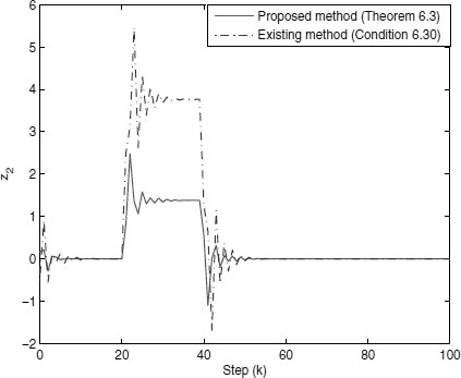
FIGURE 6.2
Comparison of the regulated output responses of z₂(t) with θ_a = 0.006.

From this example, we can see that the worst case (s_a = 15) of Theorem 6.3 also is more effective than the non-fragile Hcontroller existence condition (6.30).