6.3    Non-Fragile H_∞ Controller Design for Continuous-Time Systems

In this section, the non-fragile dynamic output feedback H_∞ controller design for continuous-time systems with the interval type of gain variations is considered.

6.3.1    Problem Statement

Consider a continuous-time linear time-invariant model described by

$\begin{array}{lll}\dot{x}\left(t\right)\hfill & =\hfill & Ax\left(t\right)+B_1\omega \left(t\right)+B_{2}u\left(t\right),\hfill \\ z\left(t\right)\hfill & =\hfill & C_{1}x\left(t\right)+D_{12}u\left(t\right),\hfill \\ y\left(t\right)\hfill & =\hfill & C_{2}x\left(t\right)+D_{12}\omega \left(t\right),\hfill \end{array}$

(6.38)

where x(t) ∈ Rⁿ is the state, u(t) ∈ R^m is the control input, y(t) ∈ R^p is the measured output, ω(t) ∈ R^r is the disturbance input, z(t) ∈ R^q is the regulated output, and A, B₁, B₂, C₁, C₂, D₁₂, and D₂₁ are known constant matrices of appropriate dimensions.

And for system (6.38), consider a dynamic output feedback controller with gain variations of the following form:

$\begin{array}{lll}\dot{\xi }\left(t\right)\hfill & =\hfill & \left(A_k+\text{Δ}{A}_k\right)\xi \left(t\right)+\left(B_k+\text{Δ}{B}_k\right)y\left(t\right),\hfill \\ u\left(t\right)\hfill & =\hfill & \left(C_k+\text{Δ}{C}_k\right)\xi \left(t\right),\hfill \end{array}$

(6.39)

where ξ(t) ∈ Rⁿ is the controller state, and A_k, B_k, and C_k are controller gain matrices of appropriate dimensions to be designed. ΔA_k, ΔB_k, and ΔC_k represent the additive gain variations of the interval type (6.3).

6.3.2    Non-Fragile H_∞ Controller Design Methods

Note that the proofs of the main results are similar to those of discrete-time systems, so here we only give the main results for continuous-time systems without proofs.

First, we give the design method of the initial controller gain C_k, which will be used in the non-fragile H_∞ controller design.

Consider the controller (6.39) with ΔA_k = 0 and ΔB_k = 0, which is described by

$\begin{array}{lll}\dot{\xi }\left(t\right)\hfill & =\hfill & A_k\text{ξ}\left(t\right)+B_{k}y\left(t\right)\hfill \\ u\left(t\right)\hfill & =\hfill & \left(C_k+\text{Δ}{C}_k\right)\text{ξ}\left(t\right),\hfill \end{array}$

(6.40)

where ΔC_k is with the norm-bounded form as in the discrete-time case of the former section.

Combining the controller (6.40) with the system (6.38), we obtain the following closed-loop system:

$\begin{array}{lll}{\dot{x}}_e\left(t\right)\hfill & =\hfill & A_{edc}{x}_e\left(t\right)+B_{edc}\omega \left(t\right)\hfill \\ z\left(t\right)\hfill & =\hfill & C_e{x}_e\left(t\right),\hfill \end{array}$

(6.41)

Then the following theorem gives a design method of the initial controller gain C_k.

Theorem 6.4 Consider system (6.38), where γ > 0 and θ_a > 0 are constants. If there exist matrices $\widehat{A},\widehat{B},\widehat{C},X>0,$ and Y > 0, and a constant ε_c > 0 such that the following LMI holds:

$\begin{array}{c}[\begin{array}{llll}{\text{Σ}}_1\hfill & A+\widehat{A}\hfill & B_1\hfill & X{C}_1^T+{\widehat{C}}^T{D}_{12}^T\hfill \\ \ast \hfill & {\text{Σ}}_2\hfill & Y{B}_1+\widehat{B}{D}_{21}\hfill & C_1^T\hfill \\ \ast \hfill & \ast \hfill & -{\gamma }^{2}I\hfill & 0\hfill \\ \ast \hfill & \ast \hfill & \ast \hfill & -I\hfill \\ \ast \hfill & \ast \hfill & \ast \hfill & \ast \hfill \\ \ast \hfill & \ast \hfill & \ast \hfill & \ast \hfill \end{array}\\ \begin{array}{ll}{B}_2{M}_c\hfill & {\epsilon }_c{\theta }_{a}X{E}_c^T\hfill \\ Y{B}_2{M}_c\hfill & 0\hfill \\ 0\hfill & 0\hfill \\ D_{12}{M}_c\hfill & 0\hfill \\ -{\epsilon }_{c}I\hfill & 0\hfill \\ \ast \hfill & -{\epsilon }_{c}I\hfill \end{array}]<0,\end{array}$

(6.42)

where ${\text{Σ}}_1=AX+B_2\widehat{C}+X{A}^T+{\widehat{C}}^T{B}_2^T\text{ and }{\text{Σ}}_2=YA+\widehat{B}{C}_2+A^{T}Y+C_2^T{\widehat{B}}^T,$ then the controller (6.40) with

$\begin{array}{lll}{A}_k\hfill & =\hfill & {\left(X^{-1}-Y\right)}^{-1}\left(\widehat{A}-YAX-\widehat{B}{C}_{2}X-Y{B}_2\widehat{C}\right)X^{-1},\hfill \\ B_k\hfill & =\hfill & {\left(X^{-1}-Y\right)}^{-1}\widehat{B},C_k=\widehat{C}{X}^{-1}\hfill \end{array}$

(6.43)

solves the non-fragile H_∞ control problem for system (6.38).

Then, with the initial controller gain C_k designed above, we give the non-fragile dynamic output feedback H_∞ controller design methods in the following.

Theorem 6.5 Consider the plant (6.38), where γ > 0 and θ_a > 0 are given constants, and the gain matrix C_k is given. If there exist matrices F_A, F_B, S_a > 0, N_a < 0, such that the following LMIs hold:

$\begin{array}{c}{M}_0\left(\text{Δ}{A}_k,\text{Δ}{B}_k,\text{Δ}{C}_k\right)<0,{\theta }_{aij},{\theta }_{bit},{\theta }_{clj}\in \left\{-{\theta }_a,{\theta }_a\right\},\\ i,j=1,\cdots ,n; t=1,\cdots ,p; l=1,\cdots ,m,\end{array}$

(6.44)

then the controller (6.39) with additive uncertainty described by (6.3), C_k, and

$A_k=N_a^{-1}{F}_A,B_k=N_a^{-1}{F}_B$

(6.45)

solves the non-fragile H_∞ control problem for system (6.38), where

$M_0\left(\text{Δ}{A}_k,\text{Δ}{B}_k,\text{Δ}{C}_k\right)=\left[\begin{array}{ccc}{M}_{0a}+M_{0a}^T& M_{0b}& M_{0c}^T\\ \ast & -{\gamma }^{2}I& 0\\ \ast & \ast & -I\end{array}\right],$

(6.46)

with

$\begin{array}{c}{M}_{0a}=[\begin{array}{c}{S}_{a}A+S_a{B}_2\left(C_k+\text{Δ}{C}_k\right)\\ {\text{Φ}}_1+\left(S_a-N_a\right)A+F_B{C}_2+N_a\text{Δ}{B}_k{C}_2\end{array}\\ \begin{array}{c}{S}_{a}A\\ \left(S_a-N_a\right)A+F_B{C}_2+N_a\text{Δ}{B}_k{C}_2\end{array}],\end{array}$

$M_{0b}=\left[\begin{array}{c}{S}_a{B}_1\\ \left(S_a-N_a\right)B_1+F_B{D}_{21}+N_a\text{Δ}{B}_k{D}_{21}\end{array}\right],$

$M_{0c}=\left[\begin{array}{cc}{C}_1+D_{12}\left(C_k+\text{Δ}{C}_k\right)& C_1\end{array}\right],$

and Φ₁ = F_A + N_aΔA_k + (S_a – N_a)B₂(C_k + ΔC_k).

Similar to the discrete-time case, it should be noted that the number of LMIs involved in (6.44) is 2^{n2 + np + nq}, which results in the difficulty of implementing the LMI constraints in computation. To overcome the difficulty arising from implementing the design condition given in Theorem 6.5, the following method is developed.

Denote

$\begin{array}{lll}{F}_{a1}\hfill & =\hfill & \left[\begin{array}{llll}{f}_{a11}\hfill & f_{a12}\hfill & \mathrm{\cdots }\hfill & f_{a1l_a}\hfill \end{array}\right],\hfill \\ F_{a2}\hfill & =\hfill & {\left[\begin{array}{cccc}{f}_{a21}^T& f_{a22}^T& \mathrm{\cdots }& f_{a2l_a}^T\end{array}\right]}^T\hfill \end{array}$

(6.47)

where l_a = n² + np + nm, and

$\begin{array}{lll}{f}_{a1k}\hfill & =\hfill & {\left[\begin{array}{cccc}{0}_{1\times n}& {\left(N_a{e}_i\right)}^T& 0_{1\times r}& 0_{1\times q}\end{array}\right]}^T,\hfill \\ f_{a2k}\hfill & =\hfill & \left[\begin{array}{cccc}{e}_i^T& 0_{1\times n}& 0_{1\times r}& 0_{1\times q}\end{array}\right],\hfill \\ \text{for }k\hfill & =\hfill & \left(i-1\right)n+j,i,j=1,\mathrm{\cdots },n.\hfill \\ f_{a1k}\hfill & =\hfill & {\left[\begin{array}{cccc}{0}_{1\times n}& {\left(N_a{e}_i\right)}^T& 0_{1\times r}& 0_{1\times q}\end{array}\right]}^T,\hfill \\ f_{a2k}\hfill & =\hfill & \left[\begin{array}{cccc}{h}_j^T{C}_2& h_j^T{C}_2& h_j^T{D}_{21}& 0_{1\times q}\end{array}\right],\hfill \\ \text{for }k\hfill & =\hfill & n^2+\left(i-1\right)p+j,i=1,\mathrm{\cdots },n,j=1,\mathrm{\cdots },p.\hfill \\ f_{a1k}\hfill & =\hfill & {\left[\begin{array}{cccc}{\left(S_a{B}_{2gi}\right)}^T& {\left[\left(S_a-N_a\right)B_{2gi}\right]}^T& 0_{1\times r}& {\left(D_{12gi}\right)}^T\end{array}\right]}^T,\hfill \\ f_{a2k}\hfill & =\hfill & \left[\begin{array}{cccc}{e}_j^T& 0_{1\times n}& 0_{1\times r}& 0_{1\times q}\end{array}\right],\hfill \\ \text{for }k\hfill & =\hfill & n^2+np+\left(i-1\right)n+j,i=1,\mathrm{\cdots },m,j=1,\mathrm{\cdots },n.\hfill \end{array}$

Let k₀, k₁, …, k_Sa be integers satisfying

$k_0=0<k_1<\mathrm{\cdots }<k_{s_a}=l_a$

(6.48)

and matrix Σ have the following structure,

$\sum =\left[\begin{array}{cc}diag\left[{\sigma }_{11}^1\mathrm{\cdots }{\sigma }_{11}^{s_a}\right]& diag\left[{\sigma }_{12}^1\mathrm{\cdots }{\sigma }_{12}^{s_a}\right]\\ diag\left[{\sigma }_{12}^1\mathrm{\cdots }{\sigma }_{12}^{s_a}\right]& diag\left[{\sigma }_{22}^1\mathrm{\cdots }{\sigma }_{22}^{s_a}\right]\end{array}\right],$

(6.49)

where ${\sigma }_{11}^i,{\sigma }_{12}^i,$ and ${\sigma }_{22}^i\in R^{\left(k_i-k_{i-1}\right)\times \left(k_i-k_{i-1}\right)},i=1,\cdots ,s_a$.

Theorem 6.6 Consider the plant (6.38), where γ > 0, θ_a > 0, and s_a > 0 are given constants, and the gain matrix C_k is given. If there exist matrices F_A, F_B, S_a > 0, N_a < 0, and symmetric matrix Σ with the structure described by (6.49) such that the following LMIs hold:

$\left[\begin{array}{cc}Q& F_{a1}\\ F_{a1}^T& 0\end{array}\right]+{\left[\begin{array}{cc}{F}_{a2}& 0\\ 0& I\end{array}\right]}^T\sum \left[\begin{array}{cc}{F}_{a2}& 0\\ 0& I\end{array}\right]<0,$

(6.50)

$\begin{array}{l}{\left[\begin{array}{c}I\\ diag\left[{\theta }_{k_{t-1}+j}\cdots {\theta }_{k_t}\right]\end{array}\right]}^T\left[\begin{array}{cc}{\sigma }_{11}^i& {\sigma }_{12}^i\\ {\left({\sigma }_{12}^i\right)}^T& {\sigma }_{22}^i\end{array}\right]\hfill \\ \times \left[\begin{array}{c}I\\ diag\left[{\theta }_{k_{t-1}+j}\cdots {\theta }_{k_t}\right]\end{array}\right]\ge 0,\text{ for all }{\theta }_{k_{t-1}+j}\in \left\{-{\theta }_a,{\theta }_a\right\}\hfill \\ j=1,\cdots ,k_i-k_{i-1},i=1,\cdots ,s_{a,}\hfill \end{array}$

(6.51)

where

$\begin{array}{c}Q=\left[\begin{array}{ccc}{M}_{as}+M_{as}^T& M_{bs}& M_{cs}^T\\ \ast & -{\gamma }^{2}I& 0\\ \ast & \ast & -I\end{array}\right],\\ M_{as}=\left[\begin{array}{cc}{S}_{a}A+S_a{B}_2{C}_k& S_{a}A\\ \left(S_a-N_a\right)A+F_B{C}_2+{\text{Φ}}_3& \left(S_a-N_a\right)A+F_B{C}_2\end{array}\right],\\ M_{bs}=\left[\begin{array}{c}{S}_a{B}_1\\ \left(S_a-N_a\right)B_1+F_B{D}_{21}\end{array}\right],M_{cs}=\left[\begin{array}{cc}{C}_1+D_{12}{C}_k& C_1\end{array}\right],\end{array}$

(6.52)

with Φ₃ = F_A + (S_a – N_a)B₂C_k.

Then (6.39) with additive uncertainty described by (6.3), C_k, and the controller gain parameters given by (6.45) solve the non-fragile H_∞ control problem for system (6.38).

Remark 6.7 In Theorem 6.6, in some cases, the magnitude of the designed A_k (B_k) may be too large to be applied in practice. For solving the problem, in Theorem 6.6, by adding the following constraints

$N_a<-\alpha I,F_A{F}_A^T<\beta I,$

(6.53)

then the magnitude of A_k can be reduced. In fact, by $A_k=N_a^{-1}{F}_A$ and (6.53), it follows that

$\Vert A_F\Vert <1/\alpha \Vert F_A\Vert \le \sqrt{\beta }/\alpha .$

The same method can be applied for the gain B_k.

In the following, we will introduce the result of non-fragile H_∞ controller design with norm-bounded gain variations with the form (6.29), and the relationship with our result is discussed.

Noting that the problem of non-fragile dynamic output feedback H_∞ controller design with norm-bounded gain variations is also a non-convex problem, and similar to Theorem 6.6, when the controller gain C_k is known it is converted to a convex one. First, assume C_k is known. Then, by using the method in Yang, Wang, and Lin [149] and Mahmoud [103], the non-fragile H_∞ controller design with norm-bounded gain variations is reduced to solve the following LMI:

$\left[\begin{array}{ccc}Q& M_{a1}& {\theta }_a\epsilon M_{a2}^T\\ \ast & -\epsilon I& 0\\ \ast & \ast & -\epsilon I\end{array}\right]<0,$

(6.54)

with S_a > 0 and N_a < 0, where Q is defined by (6.52) with known C_k, ε > 0 is a given scalar, and

$\begin{array}{c}{M}_{a1}=[\begin{array}{cccc}{S}_a{B}_2{M}_c& 0& 0& 0\\ 0& N_a{M}_a& N_a{M}_b& S_a{B}_2{M}_c\\ 0& 0& 0& 0\\ 0& 0& 0& 0\end{array}\\ \begin{array}{ll}0\hfill & 0\hfill \\ -N_a{B}_2{M}_c\hfill & 0\hfill \\ 0\hfill & 0\hfill \\ 0\hfill & D_{12}{M}_c\hfill \end{array}],\end{array}$

$M_{a2}=\left[\begin{array}{llll}{E}_c\hfill & 0\hfill & 0\hfill & 0\hfill \\ E_a\hfill & 0\hfill & 0\hfill & 0\hfill \\ E_b{C}_2\hfill & E_b{C}_2\hfill & E_b{D}_{21}\hfill & 0\hfill \\ E_c\hfill & 0\hfill & 0\hfill & 0\hfill \\ E_c\hfill & 0\hfill & 0\hfill & 0\hfill \\ E_c\hfill & 0\hfill & 0\hfill & 0\hfill \end{array}\right].$

The following lemma will show the relationship between condition (6.54) and the condition for designing non-fragile H_∞ controllers given in Theorem 6.6.

Lemma 6.3 Consider the system (6.38). If condition (6.54) is feasible, then the condition for designing non-fragile H_∞ controllers given in Theorem 6.6 is feasible.

Combining the results in Theorem 6.4 and Theorem 6.6, we have the following algorithm.

Algorithm 6.2

Step 1. Minimize γ subject to X > 0, Y > 0, and LMI (6.42). Denote the optimal solutions as X = X_opt and $\widehat{C}={\widehat{C}}_{opt}$ Then by (6.43), $C_{kopt}={\widehat{C}}_{opt}{X}_{opt}^{-1}$

Step 2. Let C_k = C_kopt, minimize γ subject to F_A, F_B, N_a > 0, S_a > 0, and LMIs (6.50) and (6.51). Denote the optimal solutions as N_a = N_aopt, F_A = F_Aopt, and F_B = F_Bopt. Then according to (6.45), we obtain $A_k=N_a^{-1}{F}_{Aopt}$, $B_k=N_a^{-1}{F}_{Bopt}$. The resulting A_k, B_k, and C_k will form the non-fragile dynamic output feedback H_∞ controller gains.

In Theorem 6.6, we restrict the Lyapunov function matrix P with the structure (2.14) for obtaining the convex design condition, which may result in more conservative evaluation of the H_∞ performance index bound. So, in this section, for a designed controller, the Lyapunov matrix P without the restriction is exploited for obtaining less conservative evaluation of the H_∞ performance index bound.

When the controller parameter matrices A_k, B_k, and C_k are known, the problem of minimizing γ subject to (6.3) for a given θ_a > 0 and ‖ T_Zeω‖< γ can be converted into the one: minimize γ² subject to the following LMIs:

$\begin{array}{l}\left[\begin{array}{ccc}P{A}_e+A_e^{T}P& P{B}_e& C_e^T\\ \ast & -{\gamma }^{2}I& 0\\ \ast & \ast & -I\end{array}\right]<0,{\theta }_{aij},{\theta }_{bit},\theta clj\in \left\{-{\theta }_a,{\theta }_a\right\},\hfill \\ i,j=1,\cdots ,n;t=1,\cdots ,p;l=1,\cdots ,m.\hfill \end{array}$

(6.55)

Similar to the design condition given in Theorem 6.5, the above optimization problem is also with the numerical computational problem, to solve the problem, the following lemma provides a solution using the structured vertex separator approach.

Denote

$\begin{array}{r}\hfill G_{a1}=\left[\begin{array}{cccc}{g}_{a11}& g_{a12}& \cdots & g_{a1l_a}\end{array}\right],\\ \hfill G_{a2}={\left[\begin{array}{cccc}{g}_{a21}^T& g_{a22}^T& \cdots & g_{a2l_a}^T\end{array}\right]}^T,\end{array}$

(6.56)

where

$\begin{array}{lll}{g}_{a1k}\hfill & =\hfill & {\left[\begin{array}{lll}\left[\begin{array}{cc}{0}_{1\times n}& e_i^T\end{array}\right]P\hfill & 0_{1\times r}\hfill & 0_{1\times q}\hfill \end{array}\right]}^T,\hfill \\ g_{a2k}\hfill & =\hfill & \left[\begin{array}{llll}{0}_{1\times n}\hfill & e_j^T\hfill & 0_{1\times r}\hfill & 0_{1\times q}\hfill \end{array}\right],\hfill \\ \text{for }k\hfill & =\hfill & \left(i-1\right)n+j,i,j=1,\cdots ,n.\hfill \\ g_{a1k}\hfill & =\hfill & {\left[\begin{array}{lll}\left[\begin{array}{cc}{0}_{1\times n}& e_i^T\end{array}\right]P\hfill & 0_{1\times r}\hfill & 0_{1\times q}\hfill \end{array}\right]}^T,\hfill \\ g_{a2k}\hfill & =\hfill & \left[\begin{array}{llll}{h}_j^T{C}_2\hfill & 0_{1\times n}\hfill & h_j^T{D}_{21}\hfill & 0_{1\times q}\hfill \end{array}\right],\hfill \\ \text{for }k\hfill & =\hfill & n^2+\left(i-1\right)p+j,i=1,\cdots ,n,j=1,\cdots ,p.\hfill \\ g_{a1k}\hfill & =\hfill & {\left[\begin{array}{llll}\left[\begin{array}{ll}{\left(B_2{g}_i\right)}^T\hfill & 0_{1\times n}\hfill \end{array}\right]P\hfill & 0_{1\times n}\hfill & 0_{1\times r}\hfill & {\left(D_{12}{g}_i\right)}^T\hfill \end{array}\right]}^T,\hfill \\ g_{a2k}\hfill & =\hfill & \left[\begin{array}{llll}{0}_{1\times n}\hfill & e_j^T\hfill & 0_{1\times r}\hfill & 0_{1\times q}\hfill \end{array}\right]\hfill \\ \text{for }k\hfill & =\hfill & n^2+np+\left(i-1\right)n+j,i=1,\cdots ,m,j=1,\cdots ,n.\hfill \end{array}$

Then we have the following lemma.

Lemma 6.4 Consider the system (6.38). Let γ > 0 and θ_a > 0 be constants, and let controller parameter matrices A_k, B_k, and C_k be given. Then ‖ T_zω ‖< γ holds for all θ_aij, θ_bit, and θ_clj satisfying (6.3), if there exist matrices P > 0 and symmetric matrix Σ with the structure described by (6.49) such that (6.51) and the following LMI hold:

$\left[\begin{array}{cc}{Q}_s& G_{a1}\\ G_{a1}^T& 0\end{array}\right]+{\left[\begin{array}{cc}{G}_{a2}& 0\\ 0& I\end{array}\right]}^T\sum \left[\begin{array}{cc}{G}_{a2}& 0\\ 0& I\end{array}\right]<0$

(6.57)

where

$\begin{array}{c}{Q}_s=[\begin{array}{c}P\left[\begin{array}{cc}A& B_2{C}_k\\ B_k{C}_2& A_k\end{array}\right]+{\left[\begin{array}{cc}A& B_2{C}_k\\ B_k{C}_2& A_k\end{array}\right]}^{T}P\\ \ast \\ \ast \end{array}\\ \begin{array}{ll}P\left[\begin{array}{c}{B}_1\\ B_k{D}_{21}\end{array}\right]\hfill & \left[\begin{array}{c}{C}_1^T\\ {\left(D_{12}{C}_k\right)}^T\end{array}\right]\hfill \\ -{\gamma }^{2}I\hfill & 0\hfill \\ \ast \hfill & -I\hfill \end{array}].\end{array}$

(6.58)

Remark 6.8 For evaluating the H_∞ performance bound of the transfer function from ω to z, the condition given in Lemma 6.4 usually is less conservative than that given in Theorem 6.6 because no structure constraint on the Lyapunov function matrix in Lemma 6.4 is imposed.

6.3.3    Example

To illustrate the effectiveness of the proposed non-fragile H_∞ controller, an example is given to provide a comparison between the proposed non-fragile H_∞ controller design method and the existing non-fragile H_∞ controller design method with the norm-bounded gain variations. Consider a linear system of the form (6.38) with

$\begin{array}{c}A=\left[\begin{array}{lll}0\hfill & 1\hfill & 0\hfill \\ 0\hfill & -1\hfill & -1\hfill \\ 0\hfill & 1\hfill & -1\hfill \end{array}\right],B_1=\left[\begin{array}{ll}-1\hfill & 0\hfill \\ 1\hfill & 0\hfill \\ 1\hfill & 0\hfill \end{array}\right],B_2=\left[\begin{array}{l}1\hfill \\ 2\hfill \\ -2\hfill \end{array}\right],\\ C_1=\left[\begin{array}{lll}2\hfill & -1\hfill & -2\hfill \\ 0\hfill & 0\hfill & 0\hfill \end{array}\right],C_2=\left[\begin{array}{lll}-2\hfill & 2\hfill & -1\hfill \end{array}\right],\\ D_{21}=\left[\begin{array}{ll}0\hfill & 0.5\hfill \end{array}\right],D_{12}=\left[\begin{array}{l}0\hfill \\ 1\hfill \end{array}\right].\end{array}$

By the standard H_∞ controller design method [113], we obtain the optimal H_∞ performance index for the system as γ_opt = 2.7069.

On the other hand, assume that the designed controller is in the form of (6.40). Let θ_a = 0.05, then by Theorem 6.3 with ε_c = 0.0023, we obtain

$C_{k_{ini}}=\left[-3.0525\text{ 0}\text{.0998 1}\text{.3036}\right].$

Here, ε_c is obtained by searching such that the H_∞ performance index is optimal. The value for θ_a is chosen appropriately large such that the designed C_kini can guarantee that Step 2 is feasible.

In the following, we design an H_∞ controller by condition (6.54) with C_k = C_kini

Assume that the designed controller is with norm-bounded additive uncertainties described by (6.29), by applying condition (6.54) with θ_a = 0.02 and ε_c = 0.0040 to design a non-fragile controller. The obtained gains are given by

$\begin{array}{lll}{A}_{K_{nm}}\hfill & =\hfill & {10}^8\times \left[\begin{array}{lll}-2.0220\hfill & 2.0588\hfill & -0.9508\hfill \\ -0.9435\hfill & 0.9607\hfill & -0.4436\hfill \\ 1.0268\hfill & -1.0455\hfill & 0.4828\hfill \end{array}\right],\hfill \\ B_{K_{nm}}\hfill & =\hfill & {10}^8\times {\left[\begin{array}{lll}-1.0030\hfill & -0.4680\hfill & 0.5093\hfill \end{array}\right]}^T,\hfill \end{array}$

and the H_∞ performance index of the obtained non-fragile controller is 3.3719. Note that the ε_c used here is obtained by the searching method to guarantee the H_∞ performance index is optimal.

Notice that the gains of the above controller are too large to be applied in practice. As indicated in Remark 6.7, applying condition (6.54) with (6.53), and with α = 0.4 and β = 1000000, the controller gains are reduced as:

$\begin{array}{lll}{A}_{K_{nm}}\hfill & =\hfill & \left[\begin{array}{lll}-93.7030\hfill & 93.1259\hfill & -41.7578\hfill \\ -45.8612\hfill & 39.1903\hfill & -16.4768\hfill \\ 48.3981\hfill & -42.3883\hfill & 16.5820\hfill \end{array}\right],\hfill \\ B_{K_{nm}}\hfill & =\hfill & {\left[\begin{array}{lll}-45.0240\hfill & -19.3069\hfill & 21.1626\hfill \end{array}\right]}^T,\hfill \end{array}$

and the H_∞ performance index is 3.4514.

Then, we design an H_∞ controller by Theorem 6.6 with C_k = C_kini.

Assume that the designed controller is with the additive interval type of uncertainties described by (6.3). For this case with C_k = C_kini, it is difficult to apply Theorem 6.5 to design a non-fragile H_∞ controller because the number of the LMI constraints involved in (6.44) is 2¹⁵. However, Theorem 6.6 is applicable for solving this problem. By applying Theorem 6.6 with θ_a = 0.02 and k_i = i, i = 1, …, 15, that is, s_a = 15 as well as k_i = 3i, i = 1, …, 5, that is, s_a = 5 to design a non-fragile controller, the obtained gains are as follows.

For s_a = 15,

$\begin{array}{lll}{A}_K\hfill & =\hfill & {10}^7\times \left[\begin{array}{lll}-9.5028\hfill & 9.4661\hfill & -4.4679\hfill \\ -3.3994\hfill & 3.3863\hfill & -1.5983\hfill \\ 6.2383\hfill & -6.2142\hfill & 2.9330\hfill \end{array}\right],\hfill \\ B_k\hfill & =\hfill & {10}^7\times {\left[\begin{array}{lll}-4.6909\hfill & -1.6781\hfill & 3.0794\hfill \end{array}\right]}^T.\hfill \end{array}$

For s_a = 5,

$\begin{array}{lll}{A}_K\hfill & =\hfill & {10}^8\times \left[\begin{array}{lll}-4.7744\hfill & 4.7522\hfill & -2.2444\hfill \\ -1.7067\hfill & 1.69888\hfill & -0.8023\hfill \\ 3.1388\hfill & -3.1243\hfill & 1.4755\hfill \end{array}\right],\hfill \\ B_k\hfill & =\hfill & {10}^8\times {\left[\begin{array}{lll}-2.3556\hfill & -0.8421\hfill & 1.5487\hfill \end{array}\right]}^T.\hfill \end{array}$

Correspondingly, the H_∞ performance indexes of the obtained non-fragile controllers are γ = 3.0598 and γ = 3.0578, respectively.

Similarly, the gains of the above two controllers are too large to be applied in practice. Applying Theorem 6.6 with (6.53), and with α = 0.4 and β = 1000000, the controller gains are reduced as follows.

For s_a = 15,

$\begin{array}{lll}{A}_k\hfill & =\hfill & \left[\begin{array}{lll}-83.1053\hfill & 81.2701\hfill & -37.0045\hfill \\ -31.4088\hfill & 24.1061\hfill & -9.5972\hfill \\ 56.8175\hfill & -50.1947\hfill & 20.7228\hfill \end{array}\right],\hfill \\ B_k\hfill & =\hfill & {\left[\begin{array}{lll}-39.8799\hfill & -12.1129\hfill & 25.4119\hfill \end{array}\right]}^T.\hfill \end{array}$

For s_a = 5,

$\begin{array}{lll}{A}_k\hfill & =\hfill & \left[\begin{array}{lll}-82.9818\hfill & 81.1005\hfill & -36.9408\hfill \\ -31.3580\hfill & 24.0411\hfill & -9.5724\hfill \\ 56.7847\hfill & -50.1297\hfill & 20.7037\hfill \end{array}\right],\hfill \\ B_k\hfill & =\hfill & {\left[\begin{array}{lll}-39.8034\hfill & -12.0838\hfill & 25.3848\hfill \end{array}\right]}^T.\hfill \end{array}$

The H_∞ performance indices of the obtained non-fragile controllers are γ = 3.0913 and γ = 3.0898, respectively. Compared with the above design without (6.53), the design results in a slight performance degradation, but the magnitude of A_k and B_k has been significantly reduced.

In the following part, for the above designed controllers, Lemma 6.4 can give better evaluations of the H_∞ performance index bounds.

First, to facilitate the presentation, denote the controller designed by condition (6.54) with (6.53) as K_nmαβ, while denoting the controllers designed by Theorem 6.6 with (6.53) as K_in15αβ (s_a = 15) and K_in5αβ (s_a = 5).

By Lemma 6.4, the H_∞ performance indices of the controller K_nmαβ are γ = 3.2945 (s_a = 15) and γ = 3.2940 (s_a = 5), while the H_∞ performance indices of the controllers K_in15αβ and K_in5αβ are γ = 3.0872 (s_a = 15) and γ = 3.0849 (s_a = 5), respectively.

Then, tables are given to provide a comparison between the two methods.

First, Table 6.3 shows the H_∞ performance indices achieved by the designs directly.

From Table 6.3, it is easy to see that compared with the optimal H_∞ performance index bound γ_opt = 2.7069, the performance index of the controller designed by condition (6.54) is degraded 24.57%. The performance indices of the controllers designed by Theorem 6.6 are degraded 13.04% (s_a = 15) and 12.96% (s_a = 5), which are much more improved than 24.57%.

TABLE 6.3
Performance Index by Design with θ_a = 0.02

	Condition (6.54)	Theorem 6.6 (sa = 15)	Theorem 6.6 (sa = 5)
γ	3.3719	3.0598	3.0578

TABLE 6.4
Performance Index by Design with θ_a = 0.02, α = 0.4, β = 1000000

	Condition (6.54)	Theorem 6.6 (sa = 15)	Theorem 6.6 (sa = 5)
γ	3.4514	3.0913	3.0898

Then, Table 6.4 shows the H_∞ performance indices achieved by the design conditions with (6.53).

We can see from Table 6.4 that compared with γ_opt = 2.7069, the performance index of the controller designed by (6.54) with (6.53) is degraded 27.51%. The performance indices of the controllers designed by Theorem 6.6 with (6.53) are degraded 14.20% (s_a = 15) and 14.15% (s_a = 5).

Finally, for the designed non-fragile controllers, Lemma 6.4 gives better performance indices, shown in Table 6.5.

Obviously, compared with γ_opt = 2.7069, by using Lemma 6.4, the H_∞ performance indices of the controller K_nmαβ are degraded 21.71% for s_a = 15 and 21.69% for s_a = 5. Correspondingly, the performance indices for the controllers K_in15αβ and K_in5αβ are degraded 14.05% for s_a = 15 and 13.96% for s_a = 5, respectively. The result shows the advantage of the new proposed method.

In this part, we will give a simulation to illustrate the effectiveness of the presented design method. Let $x\left(0\right)=\left[\begin{array}{ccc}-0.1& 0.6& -0.2\end{array}\right]$, $\xi \left(0\right)=\left[\begin{array}{ccc}-0.1& 0.5& 0.5\end{array}\right]$ And let the disturbance ω(t) be

$\omega \left(t\right)=\{\begin{array}{ll}0.5,\hfill & 15\le t\le 25\left(\text{second}\right)\hfill \\ 0\hfill & \text{otherwise}\text{.}\hfill \end{array}$

Then Figure 6.3 shows the regulated output responses of z₁ controlled by the non-fragile controllers designed by condition (6.54) with (6.53) and Theorem 6.6 with (6.53), and with α = 0.4, β = 1000000. The responses of z₂ controlled by the two non-fragile controllers are the same, and omitted here.

TABLE 6.5
Performance Evaluation by Lemma 6.4 with θ_a = 0.02

	Knmαβ	Kinαβ	Kinαβ
γ(sa = 15)	3.2945	3.2945	—
γ(sa = 5)	3.2940	—	3.0849

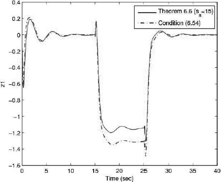
FIGURE 6.3
Comparison of the regulated output responses of z₁(t) with θ_a = 0.02.

From this example, we can see that the worst case (s_a = 15) of Theorem 6.6 also is more effective than the non-fragile H_∞ controller existence condition (6.54).

6.4    Non-Fragile H_∞ Controller Designs with Sparse Structures

6.4.1    Problem Statement

In this section, we define a class of sparse structures for controllers to be designed.

For system (6.38), consider the dynamic output feedback controller described as:

$\begin{array}{lll}\dot{\xi }\left(t\right)\hfill & =\hfill & A_k\xi \left(t\right)+B_{k}y\left(t\right),\hfill \\ u\left(t\right)\hfill & =\hfill & C_k\xi \left(t\right),\hfill \end{array}$

(6.59)

where ξ(t) ∈ Rⁿ is the controller state, and A_k, B_k, and C_k are gain matrices of appropriate dimensions.

Then, a method for finding a class of feasible sparse structures from a given fully parameterized H_∞ controller is presented as follows.

By Lemma 2.7, without loss of generality, we may assume that A_k, B_k, and C_k satisfy the following assumption:

Assumption 6.1 There exists a symmetric matrix P > 0 with the structure $P=\left[\begin{array}{cc}Y& N\\ N& -N\end{array}\right]$ such that

$A_{e0}^{T}P+P{A}_{e0}+\frac{1}{{\gamma }^2}P{B}_{e0}{B}_{e0}^{T}P+C_{e0}^T{C}_{e0}<0.$

(6.60)

Moreover, for the designed fully parameterized H_∞ controller gains A_k, B_k, and C_k, the characteristic polynomial of A_k is described as

$\det \left(sI-A_k\right)=s^n+{\alpha }_{n-1}{s}^{n-1}+\dots +{\alpha }_1+{\alpha }_0,$

(6.61)

where α₀, α₁,…, α_n–1 are scalars. Assume there exists a row vector c such that $Q={\left[\begin{array}{ccc}{\left(c{A}_k^{n-1}\right)}^T& \cdots & {\left(c{A}_k\right)}^T{c}^T\end{array}\right]}^T$ is nonsingular. Construct the following transformation matrix:

$A_{kc}=\left[\begin{array}{cccc}1& {\alpha }_{n-1}& \cdots & {\alpha }_1\\ & \ddots & \ddots & ⋮\\ & & \ddots & {\alpha }_{n-1}\\ & 0& & 1\end{array}\right]Q.$

(6.62)

Then we have that ${\overline{A}}_K,{\overline{B}}_k,\text{and }{\overline{C}}_k$ are with the following sparse structured form

$\begin{array}{lll}{\overline{A}}_k\hfill & =\hfill & T{A}_k{T}^{-1}=A_{kc}+f_A\varphi ,\hfill \\ {\overline{B}}_k\hfill & =\hfill & T{B}_k,{\overline{C}}_k=C_{k}T,\hfill \end{array}$

(6.63)

where

$\begin{array}{c}{A}_{kc}=\left[\begin{array}{cccc}0& \dots & & 0\\ 1& & & 0\\ & \ddots & & ⋮\\ 0& & 1& 0\end{array}\right],\\ f_A={\left[\begin{array}{llll}{\alpha }_0\hfill & {\alpha }_1\hfill & \cdots \hfill & {\alpha }_{n-1}\hfill \end{array}\right]}^T,\varphi =\left[\begin{array}{lll}0\hfill & \cdots \hfill & -1\hfill \end{array}\right].\end{array}$

(6.64)

Hereafter, a controller described by

$\begin{array}{lll}\dot{\overline{\xi }}\left(t\right)\hfill & =\hfill & {\overline{A}}_k\overline{\xi }\left(t\right)+{\overline{B}}_{k}y\left(t\right),\hfill \\ u\left(t\right)\hfill & =\hfill & {\overline{C}}_k\overline{\xi }\left(t\right),\hfill \end{array}$

(6.65)

with structure (6.63) is said to be a sparse structured controller.

Remark 6.9 When the gain matrices ${\overline{A}}_K,{\overline{B}}_k,\text{and }{\overline{C}}_k$ have the structure of (6.63), the nontrivial elements are only present in $f_K,{\overline{B}}_k,\text{and }{\overline{C}}_k$ So the number of additive uncertain parameters in the controller gains with any of the two structures is reduced from n²+np+mn for full parameterized controller (6.59) to n + np + mn for the sparse structured controller (6.65). Especially, when the vector c in the matrix Q is chosen from a row of C_k, denoted as C_ki, then ${\overline{C}}_{ki}=e_n^T,$ that is, the elements of the ith row of ${\overline{C}}_k$ become trivial.

Consider a sparse structured controller with gain variations described as:

$\begin{array}{lll}\dot{\overline{\xi }}\left(t\right)\hfill & =\hfill & \left({\overline{A}}_k+\text{Δ}{\overline{A}}_k\right)\overline{\xi }\left(t\right)+\left({\overline{B}}_k+\text{Δ}{\overline{B}}_k\right)y\left(t\right),\hfill \\ u\left(t\right)\hfill & =\hfill & \left({\overline{C}}_k+\text{Δ}{\overline{C}}_k\right)\overline{\xi }\left(t\right),\hfill \end{array}$

(6.66)

where $\overline{\xi }\left(t\right)\in {\text{ R}}^n$ is the controller state, and ${\overline{A}}_K,{\overline{B}}_k,\text{and }{\overline{C}}_k$ are with the structure described by (6.63). The additive gain variations $\text{Δ}{\overline{A}}_K,\text{Δ}{\overline{B}}_k,\text{and }\text{Δ}{\overline{C}}_k$ are with the following form:

$\begin{array}{lll}\text{Δ}{\overline{A}}_k=\text{Δ}{\overline{A}}_{ka}\hfill & =\hfill & {\left[{\theta }_{a\overline{a}i}\right]}_{n\times 1}v,\left|{\theta }_{a\overline{a}i}\right|\le {\theta }_a,i=1,\cdots ,n,\hfill \\ \text{Δ}{\overline{B}}_k=\text{Δ}{\overline{B}}_{ka}\hfill & =\hfill & E_{Ba}diag\left[{\theta }_{a\overline{b}1},\cdots ,{\theta }_{a\overline{b}{r}_B}\right]E_{Ba},\left|{\theta }_{a\overline{b}i}\right|\le {\theta }_a,i=1,\cdots ,r_B,\hfill \\ \text{Δ}{\overline{C}}_k=\text{Δ}{\overline{C}}_{ka}\hfill & =\hfill & E_{Ca}diag\left[{\theta }_{a\overline{c}1},\cdots ,{\theta }_{a\overline{c}{r}_C}\right]E_{Ca},\left|{\theta }_{a\overline{c}i}\right|\le {\theta }_a,i=1,\cdots ,r_C\hfill \end{array}$

(6.67)

where E_Ba, E_Bb, E_Ca, and E_Cb are constant matrices.

Remark 6.10 For the additive case, the description of the gain variations in ${\overline{B}}_k$ ${\overline{C}}_k$ given by (6.67) can cover the cases where ${\overline{B}}_k$ and ${\overline{C}}_k$ are with or without trivial elements.

Applying controller (6.66) to system (6.38), the closed-loop system is illustrated by Figure 6.4 and given by

$\begin{array}{lll}{\dot{x}}_e\left(t\right)\hfill & =\hfill & {\overline{A}}_e{\overline{x}}_e\left(t\right)+{\overline{B}}_e\omega \left(t\right),\hfill \\ z\left(t\right)\hfill & =\hfill & {\overline{C}}_e{\overline{x}}_e\left(t\right),\hfill \end{array}$

(6.68)

where ${\overline{x}}_e\left(t\right)={\left[x{\left(t\right)}^T,\overline{\xi }{\left(t\right)}^T\right]}^T$, and

$\begin{array}{lll}{\overline{A}}_e\hfill & =\hfill & \left[\begin{array}{cc}A& B_2\left({\overline{C}}_k+\text{Δ}{\overline{C}}_k\right)\\ \left({\overline{B}}_k+\text{Δ}{\overline{B}}_k\right)C_2& {\overline{A}}_k+\text{Δ}{\overline{A}}_k\end{array}\right],\hfill \\ {\overline{B}}_e\hfill & =\hfill & \left[\begin{array}{c}{B}_1\\ \left({\overline{B}}_k+\text{Δ}{\overline{B}}_k\right)D_{21}\end{array}\right],{\overline{C}}_e=\left[\begin{array}{cc}{C}_1& D_{12}\left(\left({\overline{C}}_k+\text{Δ}{\overline{C}}_k\right)\right)\end{array}\right].\hfill \end{array}$

(6.69)

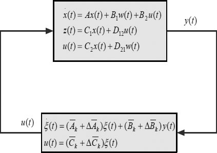
FIGURE 6.4
Control block diagram for Equation (6.68).

The transfer function matrix of the closed-loop system (6.68) from ω to z is given by

${\overline{T}}_{z\omega }={\overline{C}}_e{\left(sI-{\overline{A}}_e\right)}^{-1}{\overline{B}}_e.$

Then the problem under consideration in this chapter is as follows.

Non-fragile H_∞ control problem with sparse structure: Given positive constants γ and θ_a, design a controller described by (6.66) with additive gain variations of form (6.67) such that the resulting system (6.68) is asymptotically stable and $\Vert {\overline{T}}_{z\omega }\Vert <\gamma$.

The following preliminaries and lemmas are required in this chapter.

Lemma 6.5 Let the controller gain matrices A_k, B_k, and C_k satisfy Assumption 6.1, and T is defined by (6.62), then there exists a symmetric matrix $\overline{P}>0with\overline{P}=\left[\begin{array}{ll}\overline{Y}\hfill & \overline{N}\hfill \\ \overline{N}\hfill & -\overline{N}\hfill \end{array}\right]$ such that

${\overline{A}}_{e0}^T\overline{P}+\overline{P}{\overline{A}}_{e0}+\frac{1}{{\gamma }^2}\overline{P}{\overline{B}}_{e0}{\overline{B}}_{e0}^T\overline{P}+{\overline{C}}_{e0}^T{\overline{C}}_{e0}<0,$

(6.70)

where

$\begin{array}{c}{\overline{A}}_{e0}=\left[\begin{array}{cc}\overline{A}& {\overline{B}}_2{\overline{C}}_k\\ {\overline{B}}_k{\overline{C}}_2& {\overline{A}}_k\end{array}\right],\\ {\overline{B}}_{e0}=\left[\begin{array}{c}{\overline{B}}_1\\ {\overline{B}}_k{\overline{D}}_{21}\end{array}\right],{\overline{C}}_{e0}=\left[\begin{array}{ll}{\overline{C}}_1\hfill & {\overline{D}}_{12}{\overline{C}}_k\hfill \end{array}\right],\end{array}$

(6.71)

with ${\overline{A}}_K,{\overline{B}}_k,\text{and }{\overline{C}}_k$ given by (6.63), and

$\begin{array}{llll}\overline{A}=TA{T}^{-1},\hfill & {\overline{B}}_1=T{B}_1,\hfill & {\overline{B}}_2=T{B}_2\hfill & {\overline{C}}_1=C_1{T}^{-1},\hfill \\ {\overline{C}}_2=C_2{T}^{-1},\hfill & {\overline{D}}_{21}=D_{21}\hfill & {\overline{D}}_{12}=D_{12}.\hfill & \hfill \end{array}$

(6.72)

Proof 6.6 By Assumption 6.1, it follows that there exists a symmetric matrix P > 0 with $P=\left[\begin{array}{cc}Y& N\\ N& -N\end{array}\right]$ such that (6.60) holds. Let

$P=diag{\left[\begin{array}{cc}{T}^{-1}& T^{-1}\end{array}\right]}^{T}Pdiag\left[\begin{array}{cc}{T}^{-1}& T^{-1}\end{array}\right],$

then from (6.60), it follows that

$\begin{array}{l}{\overline{A}}_{e0}^T\overline{P}+\overline{P}{\overline{A}}_{e0}+\frac{1}{{\gamma }^2}\overline{P}{\overline{B}}_{e0}{\overline{B}}_{e0}^T\overline{P}+{\overline{C}}_{e0}^T{\overline{C}}_{e0}\hfill \\ =diag{\left[\begin{array}{cc}{T}^{-1}& T^{-1}\end{array}\right]}^T{\text{Ψ}}_{1}diag\left[\begin{array}{cc}{T}^{-1}& T^{-1}\end{array}\right]<0,\hfill \end{array}$

where ${\text{Ψ}}_1=A_{e0}^{T}P+P{A}_{e0}+\frac{1}{{\gamma }^2}P{B}_{e0}{B}_{e0}^{T}P+C_{e0}^T{C}_{e0}.$

Thus, the proof is complete.

Lemma 6.6 Let γ and θ_a be given positive constants. If there exists a symmetric matrix $\overline{P}>0with\overline{P}=\left[\begin{array}{ll}\overline{Y}\hfill & \overline{N}\hfill \\ \overline{N}\hfill & -\overline{N}\hfill \end{array}\right]$ such that

${\overline{A}}_{ea}^T\overline{P}+\overline{P}{\overline{A}}_{ea}+\frac{1}{{\gamma }^2}\overline{P}{\overline{B}}_{ea}{\overline{B}}_{ea}^T\overline{P}+{\overline{C}}_{ea}^T{\overline{C}}_{ea}<0$

(6.73)

holds for all $\text{Δ}{\overline{A}}_K,\text{Δ}{\overline{B}}_k,\text{and }\text{Δ}{\overline{C}}_k$ satisfying form (6.67), where

$\begin{array}{c}{\overline{A}}_{ea}=\left[\begin{array}{cc}\overline{A}& {\overline{B}}_2\left({\overline{C}}_k+\text{Δ}{\overline{C}}_k\right)\\ \left({\overline{B}}_k+\text{Δ}{\overline{B}}_k\right){\overline{C}}_2& {\overline{A}}_k+\text{Δ}{\overline{A}}_k\end{array}\right],\\ {\overline{B}}_{ea}=\left[\begin{array}{c}{\overline{B}}_1\\ \left({\overline{B}}_k+\text{Δ}{\overline{B}}_k\right){\overline{D}}_{21}\end{array}\right],{\overline{C}}_{ea}=\left[\begin{array}{ll}{\overline{C}}_1\hfill & {\overline{D}}_{12}\left({\overline{C}}_k+\text{Δ}{\overline{C}}_k\right)\hfill \end{array}\right],\end{array}$

(6.74)

$\overline{A},{\overline{B}}_1,{\overline{B}}_2,{\overline{C}}_1,{\overline{C}}_2,{\overline{D}}_{12},and{\overline{D}}_{21}$ are defined by (6.72). Then the controller-described by (6.66) with additive gain variations (6.67) solves the non-fragile H_∞ control problem with sparse structure for system (6.38).

Proof 6.7 Let ${\overline{P}}_s=diag{\left[\begin{array}{cc}T& I\end{array}\right]}^T\overline{P}diag\left[\begin{array}{cc}T& I\end{array}\right]$. According to (6.71), (6.72), (6.73), (6.74), it follows that

$\begin{array}{l}{\overline{A}}_e^T{\overline{P}}_s+{\overline{P}}_s{\overline{A}}_e+\frac{1}{{\gamma }^2}{\overline{P}}_s{\overline{B}}_e{\overline{B}}_e^T{\overline{P}}_s+{\overline{C}}_e^T{\overline{C}}_e\hfill \\ =diag{\left[\begin{array}{cc}T& I\end{array}\right]}^T{\text{Ψ}}_{2}diag\left[\begin{array}{cc}T& I\end{array}\right]<0,\hfill \end{array}$

where ${\text{Ψ}}_2={\overline{A}}_{ea}^T\overline{P}+\overline{P}{\overline{A}}_{ea}+\frac{1}{{\gamma }^2}\overline{P}{\overline{B}}_{ea}{\overline{B}}_{ea}^T\overline{P}+{\overline{C}}_{ea}^T{\overline{C}}_{ea}and{\overline{A}}_e,{\overline{B}}_e,{\overline{C}}_e$ are defined by (6.69). Then, by Lemma 2.6, the conclusion follows.

6.4.2    Sparse Structured Controller Design

In this section, a three-step procedure for designing non-fragile H_∞ controllers with the sparse structure with respect to additive gain uncertainties is presented.

First, we will give a method for designing a non-fragile H_∞ controller with a sparse structure (6.63) and with additive gain variations (6.67) under the assumption that the controller gain ${\overline{C}}_k$ is known.

To facilitate the presentation of Theorem 6.7, we denote

$M_{0s}\left(\text{Δ}{\overline{A}}_k,\text{Δ}{\overline{B}}_k,\text{Δ}{\overline{C}}_k\right)=\left[\begin{array}{ccc}{M}_{0sa}+M_{0sa}^T& M_{0sb}& M_{0sc}^T\\ \ast & -{\gamma }^{2}I& 0\\ \ast & \ast & -I\end{array}\right],$

(6.75)

where

$\begin{array}{c}{M}_{0as}=[\begin{array}{c}{\overline{S}}_a\left(\overline{A}+{\overline{B}}_{2e}{e}_n^T\right)+{\overline{S}}_a{\overline{B}}_{2r}\left({\overline{C}}_{kr}+\text{Δ}{\overline{C}}_{kr}\right)\\ \left({\overline{S}}_a-{\overline{N}}_a\right)\left(\overline{A}+{\overline{B}}_{2e}{e}_n^T\right)+\left({\overline{F}}_B+{\overline{N}}_a\text{Δ}{\overline{B}}_k\right){\overline{C}}_2+{\text{Φ}}_1\end{array}\\ \begin{array}{c}{\overline{S}}_a\overline{A}\\ \left({\overline{S}}_a-{\overline{N}}_a\right)\overline{A}+\left({\overline{F}}_B+{\overline{N}}_a\text{Δ}{\overline{B}}_k\right){\overline{C}}_k\end{array}],\end{array}$

$M_{0bs}=\left[\begin{array}{c}{\overline{S}}_a{\overline{B}}_1\\ \left({\overline{S}}_a-{\overline{N}}_a\right){\overline{B}}_1+\left({\overline{F}}_B+{\overline{N}}_a\text{Δ}{\overline{B}}_k\right){\overline{D}}_{21}\end{array}\right],$

$M_{0cs}=\left[\begin{array}{cc}{\overline{C}}_1+{\overline{D}}_{12e}{e}_n^T+{\overline{D}}_{12r}{\overline{C}}_{kr}+{\overline{D}}_{12r}\text{Δ}{\overline{C}}_{kr}& {\overline{C}}_1\end{array}\right].$

Here, ${\text{Φ}}_1={\overline{N}}_a{A}_{kc}+\left({\overline{F}}_A+{\overline{N}}_a\text{Δ}{f}_A\right)\varphi +\left({\overline{S}}_a-{\overline{N}}_a\right){\overline{B}}_{2r}\left({\overline{C}}_{kr}+\text{Δ}{\overline{C}}_{kr}\right)and\overline{A},{\overline{B}}_1,{\overline{B}}_2,{\overline{C}}_1,{\overline{C}}_2,{\overline{D}}_{12},and{\overline{D}}_{21}$ are defined by (6.72) with T defined by (6.62).

Then, by using Lemma 6.6, the following theorem presents a sufficient condition for the solvability of the non-fragile H_∞ control problem with sparse structure (6.63).

Theorem 6.7 Consider system (6.38). Let γ > 0 and θ_a > 0 be given constants. If there exist matrices ${\overline{F}}_A,{\overline{F}}_B,{\overline{S}}_a>0,and{\overline{N}}_a<0$ such that the following condition holds:

$\begin{array}{l}{M}_{0s}\left(\text{Δ}{\overline{A}}_{k_a},\text{Δ}{\overline{B}}_{k_a},\text{Δ}{\overline{C}}_{k_a}\right)<0\hfill \\ forall{\theta }_{a\overline{a}i},{\theta }_{a\overline{b}j},{\theta }_{a\overline{c}r}\in \left\{-{\theta }_a,{\theta }_a\right\},\hfill \\ i=1,\cdots ,n;j=1,\cdots ,r_B,r=1,\cdots ,r_c\hfill \end{array}$

(6.76)

then controller (6.66) with the gain variations described by (6.67), and

${\overline{A}}_k=A_{kc}+{\overline{N}}_a^{-1}{\overline{F}}_A\varphi ,{\overline{B}}_k={\overline{N}}_a^{-1}{\overline{F}}_B,{\overline{C}}_k$

(6.77)

solves the non-fragile H_∞ control problem with sparse structure for system (6.38).

Proof 6.8 By Lemma 6.6, it is sufficient to show that there exists a symmetric matrix $\overline{P}>0$ with structure (2.14), namely $\overline{P}\text{ = }\left[\begin{array}{cc}\overline{Y}& {\overline{N}}_a\\ {\overline{N}}_a& -{\overline{N}}_a\end{array}\right]$ such that

$M_1=\overline{P}{\overline{A}}_{ea}+{\overline{A}}_{ea}^T\overline{P}+\frac{1}{{\gamma }^2}\overline{P}{\overline{B}}_{ea}{\overline{B}}_{ea}^T\overline{P}+{\overline{C}}_{ea}^T{\overline{C}}_{ea}<0$

(6.78)

holds for all gain variations satisfying (6.67), where ${\overline{A}}_{ea},{\overline{B}}_{ea},and{\overline{C}}_{ea}$ are defined by (6.74). Denote ${\overline{S}}_a=\overline{Y}+{\overline{N}}_a,{\Gamma }_1=[\begin{array}{cc}I& I\\ I& 0\end{array}],then\overline{P}>0$ with the structure described by (2.14) is equivalent to ${\overline{S}}_a>0and{\overline{N}}_a<0$. Furthermore, Γ₁ is nonsingular for I > 0, and (6.78) is equivalent to

$\begin{array}{lll}{M}_2\hfill & =\hfill & {\text{Γ}}_1{M}_1{\text{Γ}}_1^T\hfill \\ \hfill & =\hfill & M_{2a}+M_{2a}^T+\frac{1}{{\gamma }^2}{M}_{2b}{M}_{2b}^T+M_{2c}^T{M}_{2c}<0,\hfill \end{array}$

(6.79)

where

$\begin{array}{c}{M}_{2a}=[\begin{array}{c}{\overline{S}}_a\overline{A}+{\overline{S}}_a{\overline{B}}_{2e}{e}_n^T+{\overline{S}}_a{\overline{B}}_{2r}\left({\overline{C}}_{kr}+\text{Δ}{\overline{C}}_{kr}\right)\\ {\overline{N}}_a\left({\overline{B}}_k+\text{Δ}{\overline{B}}_k\right){\overline{C}}_2+\left({\overline{S}}_a-{\overline{N}}_a\right)\overline{A}+{\text{Φ}}_2\end{array}\\ \begin{array}{c}{\overline{S}}_a\overline{A}\\ \left({\overline{S}}_a-{\overline{N}}_a\right)\overline{A}+{\overline{N}}_a\left({\overline{B}}_k+\text{Δ}{\overline{B}}_k\right){\overline{C}}_2\end{array}],\end{array}$

$M_{2b}=\left[\begin{array}{c}{\overline{S}}_a{\overline{B}}_1\\ \left({\overline{S}}_a-{\overline{N}}_a\right){\overline{B}}_1+{\overline{N}}_a\left({\overline{B}}_k+\text{Δ}{\overline{B}}_k\right){\overline{D}}_{21}\end{array}\right],$

$M_{2c}=\left[\begin{array}{cc}{\overline{C}}_1+{\overline{D}}_{12}{e}_n^T+{\overline{D}}_{12r}\left({\overline{C}}_{kr}+\text{Δ}{\overline{C}}_{kr}\right)& {\overline{C}}_1\end{array}\right]$

with ${\text{Φ}}_2={\overline{N}}_a{A}_{kc}+f_A\varphi +\text{Δ}{f}_A\varphi +\left({\overline{S}}_a-{\overline{N}}_a\right){\overline{B}}_{2e}{e}_n^T\left({\overline{S}}_a+{\overline{N}}_a\right){\overline{B}}_{2r}\left({\overline{C}}_{kr}+\text{Δ}{\overline{C}}_{kr}\right).$

Then, by (6.75), (6.77), and the Schur complement, it follows that (6.79) is equivalent to (6.76) with respect to additive gain variations (6.67). Thus, the proof is complete.

Remark 6.11 In Theorem 6.7, convex sufficient conditions for the solvability of the non-fragile H_∞ control problem with sparse structure (6.63) are given in terms of solutions to a set of LMIs. In fact, the result provides an LMI-based method for designing nan-fragile H_∞ controllers with the sparse structure from a given fully parameterized H_∞ controller. When the designed controller contains no gain variations, from Lemma 2.7, it follows that the design condition given in Theorem 6.7 reduces to a necessary and sufficient condition for the standard H_∞ control problem, which means that the structure constraint (2.14) on Lyapunov function matrices does not result in any conservativeness for the standard H_∞ controller design.

Here, we will show that the problem of the special case of single-input–single-output (SISO) is a convex one.

Consider the designed controller with gain matrices described by (6.63) and with additive gain variations (6.67).

To facilitate the presentation, denote

$M_{0s}\left(\text{Δ}{\overline{A}}_k,\text{Δ}{\overline{B}}_k,\text{Δ}{\overline{C}}_k\right)=\left[\begin{array}{ccc}{M}_{0sa}+M_{0sa}^T& M_{0sb}& M_{0sc}^T\\ \ast & -{\gamma }^{2}I& 0\\ \ast & \ast & -I\end{array}\right],$

(6.80)

where

$\begin{array}{c}{M}_{oas}=[\begin{array}{c}{\overline{S}}_a\overline{A}+{\overline{S}}_a{\overline{B}}_2\left({\overline{C}}_k+\text{Δ}{\overline{C}}_k\right)\\ \left({\overline{S}}_a-{\overline{N}}_a\right)\overline{A}+\left({\overline{F}}_B+{\overline{N}}_a\text{Δ}{\overline{B}}_k\right){\overline{C}}_2+{\text{Φ}}_1\end{array}\\ \begin{array}{c}{\overline{S}}_a\overline{A}\\ \left({\overline{S}}_a-{\overline{N}}_a\right)\overline{A}+\left({\overline{F}}_B+{\overline{N}}_a\text{Δ}{\overline{B}}_k\right){\overline{C}}_2\end{array}],\end{array}$

$M_{obs}=\left[\begin{array}{c}{\overline{S}}_a{\overline{B}}_1\\ \left({\overline{S}}_a-{\overline{N}}_a\right){\overline{B}}_1+\left({\overline{F}}_B+{\overline{N}}_a\text{Δ}{\overline{B}}_k\right){\overline{D}}_{21}\end{array}\right],$

$M_{ocs}=\left[\begin{array}{cc}{\overline{C}}_1+{\overline{D}}_{12}\left({\overline{C}}_k+\text{Δ}{\overline{C}}_k\right)& {\overline{C}}_1.\end{array}\right],$

Here, ${\text{Φ}}_1={\overline{N}}_a{A}_{kc}+\left({\overline{F}}_A+{\overline{N}}_a\text{Δ}{f}_A\right)\varphi +\left({\overline{S}}_a-{\overline{N}}_a\right){\overline{B}}_2\left({\overline{C}}_k+\text{Δ}{\overline{C}}_k\right)and\overline{A},{\overline{B}}_1,{\overline{B}}_2,{\overline{C}}_1,{\overline{C}}_2,{\overline{D}}_{12},and{\overline{D}}_{21}$ are defined by (6.72) with T defined by (6.62).

Then, according to Theorem 6.7, the following corollary presents a sufficient condition for the solvability of the non-fragile H_∞ control problem with the sparse structure (6.63).

Corollary 6.1 Consider system (6.38). Let γ > 0 and θ_a > 0 be given constants. If there exist matrices ${\overline{F}}_A,{\overline{F}}_B,{\overline{S}}_a>0,$ and ${\overline{N}}_a<0$ such that the following conditions hold:

$\begin{array}{c}{M}_{os}\left(\text{Δ}{\overline{A}}_{k_a},\text{Δ}{\overline{B}}_{k_a},\text{Δ}{\overline{C}}_{k_a},\right)<0,\\ forall{\theta }_{a\overline{a}i},{\theta }_{a\overline{b}j}\in \left\{-{\theta }_a,{\theta }_a\right\},\\ i=1,\cdots ,n;j=1,\cdots ,r_B,\end{array}$

(6.81)

then the controller (6.66) with the gain variations described by form (6.67), and

$\begin{array}{c}{\overline{A}}_k=A_{kc}+{\overline{N}}_a^{-1}{\overline{F}}_A\varphi ,\\ {\overline{B}}_k={\overline{N}}_a^{-1}{\overline{F}}_B,{\overline{C}}_k=\left[\begin{array}{cccc}0& \cdots & 0& 1\end{array}\right]\end{array}$

(6.82)

solves the non-fragile H_∞ control problem with sparse structure for system (6.38).

Remark 6.12 For SISO systems, the problem of non-fragile dynamic output feedback H_∞ controller design with the sparse structure can be converted to a convex one. In fact, if we construct the transformation matrix T by using A_k and C_k, we can obtain the sparse structured controller with ${\overline{C}}_k=\left[\begin{array}{cccc}1& 0& \dots & 0\end{array}\right]$, namely, ${\overline{C}}_k$ is known. So, by Theorem 6.7, the design conditions are given directly.

Due to the fact that the design method given by Theorem 6.7 is based on Assumption 6.1, we need to give methods for designing H_∞ controllers satisfying Assumption 6.1. First, the following standard H_∞ controller design method [113] is introduced.

Lemma 6.7 [113] Consider system (6.38). Let γ > 0 be a given scalar. If there exist matrices $\widehat{A},\widehat{B},\widehat{C},X>0$, and Y > 0 such that the following LMI holds:

$\begin{array}{c}[\begin{array}{cc}AX+X{A}^T+B_2\widehat{C}+{\left(B_2\widehat{C}\right)}^T& {\widehat{A}}^T+A\\ *& A^{T}Y+YA+\widehat{B}{C}_2+{\left(\widehat{B}{C}_2\right)}^T\\ *& *\\ *& *\end{array}\\ \begin{array}{cc}{B}_1& {\left(C_{1}X+D_{12}\widehat{C}\right)}^T\\ Y{B}_1+\widehat{B}{D}_{21}& C_1^T\\ -{\gamma }^{2}I& 0\\ *& -I\end{array}]<0,\end{array}$

(6.83)

then controller (6.59) with

$\begin{array}{lll}{A}_k\hfill & =\hfill & N^{-1}\left(\widehat{A}-YAX-\widehat{B}{C}_{2}X-Y{B}_2\widehat{C}\right)M^{-1},\hfill \\ B_k\hfill & =\hfill & N^{-1}\widehat{B},C_k=\widehat{C}{M}^{-1}\hfill \end{array}$

(6.84)

(2.19) holds, where MN^T = I – XY.

Then, by using Lemma 6.6, we present a design method to design H_∞ controllers satisfying Assumption 6.1.

Lemma 6.8 In Lemma 6.6, let M = X, then controller (6.59) with

$\begin{array}{lll}{A}_k\hfill & =\hfill & {\left(X^{-1}-Y\right)}^{-1}\left(\widehat{A}-YAX-\overline{B}{C}_{2}X-Y{B}_2\widehat{C}\right)X^{-1},\hfill \\ B_k\hfill & =\hfill & {\left(X^{-1}-Y\right)}^{-1}\widehat{B},C_k=\widehat{C}{X}^{-1},\hfill \end{array}$

(6.85)

(6.60) holds with $P\text{ = }\left[\begin{array}{cc}Y& X^{-1}-Y\\ X^{-1}-Y& -\left(X^{-1}-Y\right)\end{array}\right]$.

Proof 6.9 Let M = X, then, by using the arguments developed in Scherer, Gahinet, and Chilali [113], the conclusion follows.

Remark 6.13 Lemma 6.8 presents a method of designing H_∞ controllers for satisfying Assumption 6.1, which is the initial step for the following algorithm.

Based on Lemma 6.7 and Lemma 6.8, the following algorithm is presented to solve the non-fragile H_∞ control problem with sparse structures described by (6.63).

Algorithm 6.3 Let γ > 0 be a given scalar.

Step 1. Minimize γ subject to LMIs X > 0, Y > 0, and (6.83). Denote the optimal solutions as $X=X_{opt},Y=Y_{opt},\widehat{A}={\widehat{A}}_{opt},\widehat{B}={\widehat{B}}_{opt},$ and $\widehat{C}={\widehat{C}}_{opt}$. Substitute the matrices $\left(X_{opt},Y_{opt},{\widehat{A}}_{opt},{\widehat{B}}_{opt},{\widehat{C}}_{opt}\right)$ to (6.85), compute

$\begin{array}{lll}{A}_k\hfill & =\hfill & {\left(X_{opt}^{-1}-Y_{opt}\right)}^{-1}\left(\widehat{A}-Y_{opt}A{X}_{opt}-{\widehat{B}}_{opt}{C}_2{X}_{opt}-Y_{opt}{B}_2{\widehat{C}}_{opt}\right)X_{opt}^{-1},\hfill \\ B_k\hfill & =\hfill & {\left(X_{opt}^{-1}-Y_{opt}\right)}^{-1}{\widehat{B}}_{opt},C_k={\widehat{C}}_{opt}{X}_{opt}^{-1},\hfill \end{array}$

then go to Step 2.

Step 2. Combining A_k with the a row vector c (it can be a row vector C_ki of C_k) such that $Q={\left[\begin{array}{ccc}{\left(c{A}_k^{n-1}\right)}^T& \cdots & {\left(c{A}_k\right)}^T{c}^T\end{array}\right]}^T$ is nonsingular, by using (6.62), we construct a transformation matrix T. Then, compute $\overline{A},\overline{B},\overline{B},{\overline{C}}_1,{\overline{C}}_2,{\overline{D}}_{12},and{\overline{D}}_{21}$ according to (6.72), and go to Step 3.

Step 3. Let ${\overline{C}}_k$ = C_kT^–1. Minimize γ subject to ${\overline{F}}_A,{\overline{F}}_B,{\overline{N}}_a<0,{\overline{S}}_a>0,$ and LMI (6.76) for additive gain variations. Denote the optimal solutions as ${\overline{N}}_a={\overline{N}}_{aopt},F_A=F_{Aopt},$, and F_B = F_Bopt. Then, according to (6.77),

${\overline{A}}_k=A_{kc}+{\overline{N}}_{aopt}^{-1}{\overline{F}}_{Aopt}\varphi ,{\overline{B}}_k={\overline{N}}_{aopt}^{-1}{\overline{F}}_{Bopt},{\overline{C}}_k={\overline{C}}_k.$

The resulting ${\overline{A}}_k,{\overline{B}}_k,and{\overline{C}}_k$ form the sparse structured non-fragile H_∞ controller gains.

Remark 6.14 Algorithm 6.3 gives a method of designing the non-fragile H_∞ controller with sparse structure described by (6.63). In Step 1, an H_∞ controller satisfying Assumption 6.1 is designed, followed by determining the sparse structure, and then a non-fragile H_∞ controller with the sparse structure is obtained. In order to clarify the algorithm, Figure 6.5 is given to illustrate the flowchart of Algorithm 6.3.

For obtaining the convex design conditions, we restrict the Lyapunov function matrix P with structure (2.14) in Theorem 6.7, which may result in a more conservative evaluation of the H_∞ performance bounds. So, in this section, for a designed controller with the sparse structure, the Lyapunov matrix P without the restriction is exploited for obtaining a less conservative evaluation of the H_∞ performance bounds.

When the controller parameter matrices ${\overline{A}}_k,{\overline{B}}_k,$ and ${\overline{C}}_k$ are known, the following lemma presents sufficient conditions for measuring the non-fragile H_∞ performance of system (6.68).

Denote

$\begin{array}{lll}{M}_{oss}\left(\text{Δ}{\overline{A}}_{k_a},\text{Δ}{\overline{B}}_{k_a},\text{Δ}{\overline{C}}_{k_a}\right)\hfill & =\hfill & \left[\begin{array}{ccc}P{\overline{A}}_e+{\overline{A}}_e^{T}P& P{\overline{B}}_e& {\overline{C}}_e^T\\ \ast & -{\gamma }^{2}I& 0\\ \ast & \ast & -I\end{array}\right]\hfill \end{array},$

(6.86)

where ${\overline{A}}_e,{\overline{B}}_e,\text{and }{\overline{C}}_e$ are defined by (6.69).

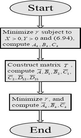
FIGURE 6.5
Flowchart of Algorithm 6.3.

Lemma 6.9 Consider system (6.38). Let γ > 0, θ_a > 0 be constants, and let controller parameter matrices ${\overline{A}}_k,{\overline{B}}_k,\text{ and}{\overline{C}}_k$ be given. Then ‖ T_zω ‖< γ holds for all gain variations described by (6.67), if there exists a symmetric matrix P > 0 such that the following condition holds:

$\begin{array}{c}{M}_{oss}\left(\text{Δ}{\overline{A}}_{k_a},\text{Δ}{\overline{B}}_{k_a},\text{Δ}{\overline{C}}_{k_a}\right)<0\\ forall{\theta }_{a\overline{a}i},{\theta }_{a\overline{b}j},\in \left\{-{\theta }_a,{\theta }_a\right\}\\ i=1,\cdots ,n;j=1,\cdots ,r_B.\end{array}$

(6.87)

6.4.3    Example

In this section, we will illustrate the effectiveness of our design methods of the non-fragile H_∞ controller with the sparse structure.

Example 6.1 Consider a linear system of form (6.38) with

$\begin{array}{c}{A}_k=\left[\begin{array}{lll}0\hfill & 1\hfill & 0\hfill \\ 0\hfill & -1\hfill & -1\hfill \\ 0\hfill & 1\hfill & -1\hfill \end{array}\right],B_1=\left[\begin{array}{ll}-1\hfill & 0\hfill \\ 0.5\hfill & 0\hfill \\ 1.5\hfill & 0\hfill \end{array}\right],B_2=\left[\begin{array}{c}1\\ 2\\ -2.5\end{array}\right],\\ C_1=\left[\begin{array}{lll}1\hfill & -1\hfill & -3\hfill \\ 0\hfill & 0\hfill & 0\hfill \end{array}\right],C_2=\left[\begin{array}{lll}-3\hfill & 2\hfill & -1\hfill \end{array}\right],\\ D_{21}=\left[\begin{array}{ll}0\hfill & 0.5\hfill \end{array}\right],D_{12}={\left[\begin{array}{ll}0\hfill & 1\hfill \end{array}\right]}^T.\end{array}$

First, by Step 1 of Algorithm 6.3, we obtain the H_∞ controller K_so with gains as

$\begin{array}{c}\begin{array}{ccc}{A}_k& =& \left[\begin{array}{lll}-20.0503\hfill & 13.3586\hfill & -2.7130\hfill \\ -4.9211\hfill & 1.3024\hfill & 4.8168\hfill \\ 26.2416\hfill & -14.4317\hfill & -1.8096\hfill \end{array}\right]\end{array},\\ \begin{array}{ccc}{B}_k& =& {\left[\begin{array}{ccc}-6.0622& -0.4246& 7.2303\end{array}\right]}^T\end{array},\\ \begin{array}{ccc}{C}_k& =& \left[\begin{array}{ccc}-1.7241& 0.6165& 2.9546\end{array}\right]\end{array},\end{array}$

and the optimal H_∞ performance is γ_opt = 2.9246.

It is easy to see that the matrix $Q={\left[{\left(C_k{A}_k^{n-1}\right)}^T\cdots {\left(C_k{A}_k\right)}^T{C}_k^T\right]}^T$ is nonsingular, so in Step 2 of Algorithm 6.3, let the row vector c = C_k. The transformation matrix is obtained as

$\begin{array}{ccc}{T}_o& =& \left[\begin{array}{lll}65.4937\hfill & 137.8543\hfill & 67.8067\hfill \\ 73.6172\hfill & -52.1905\hfill & 63.0340\hfill \\ -1.7241\hfill & 0.6165\hfill & 2.9543\hfill \end{array}\right]\end{array}.$

Then, by Step 3, when the designed sparse structured controller is assumed to be with additive uncertainties described by (6.67), by solving (6.76) with θ_a = 0.65, the non-fragile sparse structured H_∞ controller K_noa is obtained with gains as:

$\begin{array}{c}\begin{array}{ccc}{\overline{A}}_k& =& \left[\begin{array}{lll}0\hfill & 0\hfill & 56.8811\hfill \\ 1\hfill & 0\hfill & -261.3554\hfill \\ 0\hfill & 1\hfill & -40.7364\hfill \end{array}\right]\end{array},\begin{array}{ccc}{\overline{C}}_k& =& \left[\begin{array}{ccc}0& 0& 1\end{array}\right],\end{array}\\ {\overline{B}}_k={\left[\begin{array}{ccc}42.6526& 37.2199& 33.9007\end{array}\right]}^T,\end{array}$

and the H_∞ performance index is 3.4547.

On the other hand, for the designed controller K_so in Step 1 with the optimal H_∞ performance γ_opt = 2.9246, according to (6.63) and transforming k_sowith the transformation matrix T_o, we obtain the sparse structured H_∞ controller K_so1 directly with the gains as

$\begin{array}{ccc}{\overline{A}}_k& =& \left[\begin{array}{lll}0\hfill & 0\hfill & 123.0840\hfill \\ 1\hfill & 0\hfill & -214.2598\hfill \\ 0\hfill & 1\hfill & -20.5575\hfill \end{array}\right]\end{array},\begin{array}{ccc}{\overline{C}}_k& =& \left[\begin{array}{ccc}0& 0& 1\end{array}\right],\end{array}$

TABLE 6.6
Performance Evaluation of Lemma 6.9 with θ_a = 0.65

Controller	Knoa	Kso1
γ	3.2643	4.2225

TABLE 6.7
H_∞ Performance Level for Variant Values of θ_a

${\overline{B}}_k={\left[\begin{array}{ccc}34.6939& 31.6321& 31.5505\end{array}\right]}^T.$

In this part, for the above designed controllers, Lemma 6.9 gives better evaluations of the H_∞ performance index bounds, which are compared and shown in the above tables.

For the sparse structured controllers K_noa (obtained by our design Algorithm 6.3) and K_so1 (obtained by transformation with T_o directly), with θ_a = 0.65, Lemma 6.9 gives better evaluations shown in Table 6.6.

Obviously, compared with γ_opt = 2.9246, the H_∞ performance index of the controller K_noa is degraded 11.62%, while the performance index of the controller K_so1 is degraded 44.38%.

Then, a simulation is given to illustrate the effectiveness of the design method. Let $x\left(0\right)={\left[0.8\text{ -0}\text{.6 0}\text{.4}\right]}^T,\xi \left(0\right)={\left[0.3\text{ -0}\text{.5 0}\text{.8}\right]}^T$And let the disturbance ω(t) be

$\omega \left(t\right)=\{\begin{array}{ll}\left[\begin{array}{l}1\hfill \\ 1\hfill \end{array}\right],\hfill & 40\le t\le 40.5\left(second\right),\hfill \\ 0,\hfill & otherwise.\hfill \end{array}$

Then Figure 6.6 shows the regulated output responses of z₁ controlled by the sparse structured controller K_so1 (obtained by transformation with T_o directly) and the non-fragile sparse structured controller K_noa (obtained by our design Algorithm 6.3) with θ_a = 0.65, respectively. The responses of z₂ controlled by the two controllers with θ_a = 0.65 are shown in Figure 6.7. From the two figures, we can see the superiority of our proposed methods.

In the following, for variant values of θ_a, we obtain variant H_∞ performance levels by using our proposed design method as shown in Table 6.7. Figure 6.8 further presents the relationship between the H_∞ a clearly. It can be seen that, the larger the value of θ_a is, the worse the H_∞ performance level is.

FIGURE 6.6
Responses of z₁(t) with θ_a = 0.65.

FIGURE 6.7
Responses of z₂(t) with θ_a = 0.65.

FIGURE 6.8
Response of H_∞ performance (γ) with respect to θ_a.

6.5    Conclusion

The full parameterized and sparse structured non-fragile H_∞ controller design problems have been investigated in this chapter. The controller to be designed is assumed to be with the additive gain variations of interval type, which are due to the FWL effects when the controller is implemented. For the full parameterized controller design problem, we consider the discretetime and continuous-time systems, respectively. And a two-step procedure is adopted to solve this non-convex problem. In addition, the notion of a structured vertex separator is proposed to approach the numerical computational problem resulting from the interval type of gain uncertainties, and exploited to develop sufficient conditions for the non-fragile H_∞ controller design in terms of solutions to a set of LMIs. For the sparse structured controller design problem, a class of sparse structures is specified. Then, a three-step procedure for non-fragile H_∞ controller design under the restriction of the sparse structure is provided. The contribution of this method is that it not only reduces the number of nontrivial parameters but also designs the sparse structured controllers with non-fragility. The resulting designs of the two cases guarantee that the closed-loop system is asymptotically stable and the H_∞ performance from the disturbance to the regulated output is less than a prescribed level. Numerical examples are given to illustrate the effectiveness of the proposed design methods.