![]()
Graphics Special Commands
5.1 Two Dimensional Graphics: FPLOT and EZPLOT
Commands fplot and ezplot graph curves using commands developed for a wide array of cases without having to specify all the details built in every time. Their syntax is as follows:
fplot(‘f’, [xmin, xmax]) | Graphs the function between the limits in each case given in this table. |
fplot(‘f’,[xmin, xmax, ymin, ymax], S) | Graphs the function at intervals of variation of x and y , with options for color and characters given by S. ymin and ymax control the values of the vertical axis. |
fplot(‘[f1,f2,...,fn]’,[xmin, xmax, ymin, ymax], S,t,n) | Graphs functions f1, f2,..., fn on the same axes in the ranges of variation of x and specified with the options for color and characters defined in S |
fplot(‘f’,[xmin, xmax],...,t) | Graphs of f using the tolerance t |
fplot(‘f’,[xmin, xmax],...,n) | Graphs of f where n> = 1 |
ezplot(‘f’, [xmin, xmax]) | Similar to fplot |
ezplot(‘f’, [xmin, xmax, ymin, ymax]) | Graphs the function f(x,y) at given intervals of variation of x and y . Unlike fplot, ezplot can be f(x,y) |
ezplot(x, y) | Graphs the planar parametric curve x = x(t) and y = y(t) on the domain 0 < t < 2π |
ezplot(‘f’, [xmin, xmax]) | Graphs the planar parametric curve x = x(t) and y = y(t). This is a variation on ezplot(x,y) which expects two function parameters; the only difference here is that tmin and tmax are used instead of the implied 0 to 2pi. So, the syntax is ezplot(fx,fy,[tmin tmax]) |
ezplot(‘f’) | Graphs curve f in implicit in [-2π, 2π] |
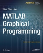
As a first example, perform the graph of the function ![]() over the range [0,10]. Figure 5-1 presents the results of the following syntax:
over the range [0,10]. Figure 5-1 presents the results of the following syntax:
>> x = 0:0.05:10;
>> y = sin(x) .* exp(-0.4*x);
>> plot(x,y)
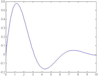
The representation of the previous curve (Figure 5-2) can also be done using the following syntax:
>> ezplot('sin(x) * exp(-0.4*x)', [0,10])
Note that ezplot automatically sets the title. You could also obtain the same graphical representation using the following command:
>> fplot('sin(x) * exp(-0.4*x)', [0,10])
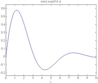
Figure 5-3 shows the curve for ![]() in the range [-2π,2π] using the following syntax:
in the range [-2π,2π] using the following syntax:
>> ezplot('x^2-y^4')
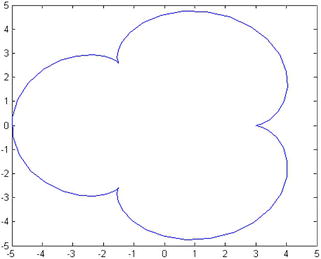
Then we graph the parametric curve– x(t) = 4cos(t) –cos(4t), y(t) = 4sin(t) –sin(4t) varying t between 0 and 2π (Figure 5-4). The syntax is as follows:
>> t = 0:0.1:2*pi;
>> x = 4 * cos(t) - cos(4*t);
>> y = 4 * sin(t) - sin(4*t);
>> plot(x,y)
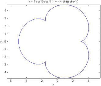
The same graph (Figure 5-5) could have been obtained by using the following syntax:
>> ezplot('4*cos(t) - cos(4*t)', '4*sin(t) - sin(4*t)', [0, 2*pi])
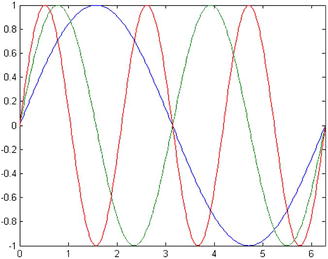
Next, were present the curves Sine (x), Sine (2x) and Sine (3x) about the same axes as shown in Figure 5-6. The syntax is as follows:
>> fplot('[sin(x), sin(2*x), sin(3*x)]', [0, 2*pi])
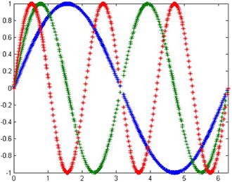
We can try to represent every previous curve using different strokes (Figure 5-7) by using the following syntax:
>> fplot('[sin(x), sin(2*x), sin(3*x)]', [0, 2*pi],'*')
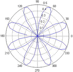
Below you will find the syntax used to represent the polar curve r = Sin (2a) Cos (2a) for t between 0 and 2π (Figure 5-8).
>> t = 0:0.1:2*pi;
>> r = sin(2*t).* cos(2*t);
>> polar(t,r)
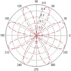
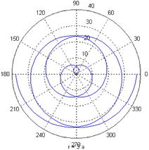
This example could also represent this polar curve with a dashed line of red color (Figure 5-9) using the following syntax:
>> t = 0:0.1:2*pi;
>> r = sin(2*t).*cos(2*t);
>> polar(t,r,'--r')
5.2 Three-Dimensional Graphics with EZ Command
In the same way that ez functions are used to represent two-dimensional graphics without specifying the field of existence of an array form, three-dimensional graphics of warped curves, surfaces, contour lines, contour and other types of graphics can also be used, the commands to use are as follows:
ezcontour(f) ezcontour(f, domain) ezcontour(...,n) | Contour graph of f(x,y) in [-2π, 2π] x [-2π, 2π] Contour graph of f(x,y) in the given domain Contour graph of f(x,y) in mesh of size n x n |
ezcontourf(f) ezcontourf(f, domain) ezcontourf(...,n) | Filling contour graph of f(x,y) in [-2π, 2π] x [-2π, 2π] Filling contour graph of f(x, y) in the given domain Contour graph of f(x, y) filling in a n x n mesh |
ezmesh(f) ezmesh(f,domain) ezmesh(...,n) ezmesh(x, y, z) ezmesh(x, y, z, domain) ezmesh(..., ‘circ’) | Filling mesh graph of f(x,y) at [-2π, 2π] x [-2π, 2π] Filling mesh raph of f(x,y) in the given domain Filling Mesh graph of f(x,y) in the nxn mesh Mesh graph for x = x(t,u), y = y(t,u), z = z(t,u) where t,u Mesh graph for x = x(t,u), y = y(t,u), z = z(t,u) where t,u Mesh graph of a circle, not the default square, centered in the domain |
ezmeshc(f) ezmeshc(f, domain) ezmeshc(...,n) ezmeshc(x, y, z) ezmeshc(x, and z, domain) ezmeshc(..., ‘circ’) | Performs a combination of mesh and contour graph elements |
ezsurf(f) ezsurf(f, domain) ezsurf(...,n) ezsurf(x, y, z) ezsurf (x, y, z, domain) ezsurf(..., ‘circ’) | These make a colored surface chart |
ezsurfc(f) ezsurfc(f, domain) ezsurfc(...,n) ezsurfc(x, y, z) ezsurfc(x, y, z, domain) ezsurfc(..., ‘circ’) | This creates diagrams that are a combination of surface and contour graphs |
ezplot3(x, y, z) ezplot3(x, y, z, domain) ezplot3(..., ‘animate’) | Parametric curve in 3D for x = x(t), y = y(t), z = z(t) t Parametric curve in 3D for x = x(t), y = y(t), z = z(t) t Parametric curve using 3D animation |
ezpolar(f) ezpolar(f, [a, b]) | Graph the polar curve r = f(c) with c Graph the polar curve r = f(c) with c |
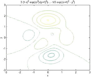
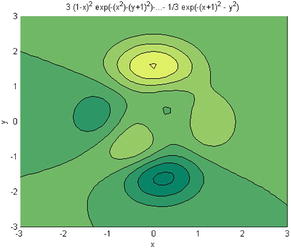
Below is the contour graph (Figure 5-10) for the function:
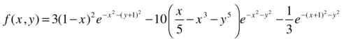
>> f = ['3 *(1-x)^2*exp(-(x^2)-(y + 1)^2)',...
'-10*(x/5-x^3-y^5)*exp(-x^2-y^2)','-1/3*exp(-(x + 1)^2 - y^2)'];

>> ezcontour(f,[-3,3],49)
   colormap summer
Then fill in color in the previous contour (Figure 5-11).
>> ezcontourf(f,[-3,3],49)
In the following example we do a mixed mesh-contour (Figure 5-12) for the chart function:
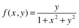
>> ezmeshc('y /(1 + x^2 + y^2)', [- 5, 5, - 2*pi, 2*pi])
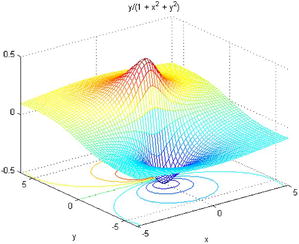
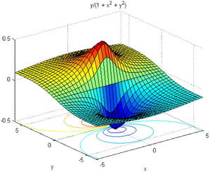
Later is a graphical surface and contour (Figure 5-13).
>> ezsurfc('y/(1 + x^2 + y^2)', [- 5, 5, - 2*pi, 2*pi], 35)
Then we graph a curve in parametric space.
>> ezplot3('sin(t)', 'cos(t)',', [0, 6 * pi])
EXERCISE 5-1
Represent the following function in the interval [–8.8]
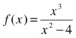
Figure 5-14 represents the function by using the following syntax:
>> ezplot('x^3 / (x^2-4)', [-8, 8])
EXERCISE 5-2
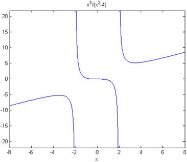
Graph, on the same axes, the functions bessel(1,x), bessel(2,x) and bessel(3,x) for values of x between 0 and 12, evenly spaced using two-tenths. Place three legends and add three different types of strokes (normal, asterisks and circles, respectively) to the three functions.
Figure 5-15 represents the capabilities requested by using the following syntax:
>> x = 0:.2:12;
plot(x, besselj(1,x), x, besselj(2,x),'*', x, besselj(3,x), 'o'),
legend('Bessel(1,x)', 'Bessel(2,x)', 'Bessel(3,x)'),
EXERCISE 5-3
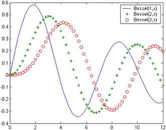
Represent the polar curve r = 4 (1 + Cos (a)) between 0 and 2π (cardioid). Also represent the curve in polar, r = 3a for a between - 4π and 4π (spiral).
The first curve (Figure 5-16) is represented using the following syntax:
>> a = 0:0.01:2*pi;
r = 4 * (1 + cos(a));
polar(a, r)
title('CARDIOID')
The second curve (Figure 5-17) can be represented using the syntax:
>> ezpolar('3*a',[-4*pi,4*pi])
EXERCISE 5-4
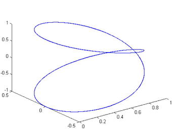
Represent the warped curve of parametric coordinates, x = Cos2(t), y = Sine (t) cos (t), z = Sine (t) for t ranging from -4π to 4π.
Figure 5-18 represents the capabilities requested by using the following syntax:
>> t = -4 * pi: 0.01:4 * pi;
x = cos(t) .^ 2;
y = sin(t) .* cos(t);
z = sin(t);
plot3(x, y, z)
EXERCISE 5-5
Represent the surface, your mesh graph and the contour graph whose equation is as follows:
![]()
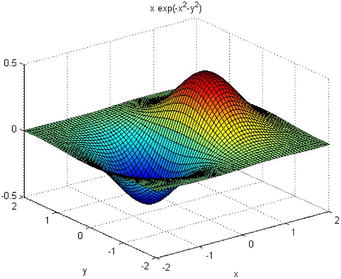
The graph of the surface (Figure 5-19) can be represented as follows:
>> ezsurf('x * exp(-x^2-y^2)', [- 2, 2], [- 2, 2])
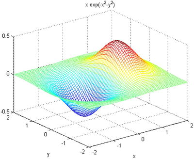
The mesh (Figure 5-20) graph can be represented as follows:
>> ezmesh('x * exp(-x^2-y^2)', [- 2, 2], [- 2, 2])
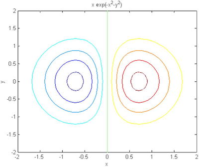
The contour graph (Figure 5-21) can be represented as follows:
>> ezcontour('x * exp(-x^2-y^2)', [-2, 2], [-2, 2])
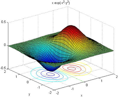
We can make the graph of the surface and contour simultaneously (Figure 5-22) as follows:
>> ezsurfc('x * exp(-x^2-y^2)', [- 2, 2], [- 2, 2])
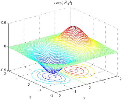
We can make the mesh-contour chart simultaneously (Figure 5-23) as follows:
>> ezmeshc('x * exp(-x^2-y^2)', [- 2, 2], [- 2, 2])
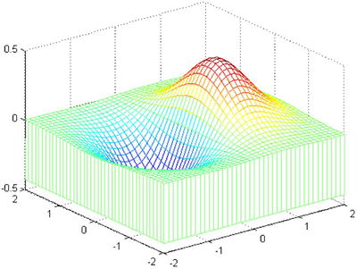
We can also represent the mesh graph with the option of curtain or curtain bottom (Figure 5-24) as follows:
>> [X, Y] = meshgrid(-2:.1:2,-2:.1:2);
Z = X .* exp(-X.^2-Y.^2);
meshz(X, Y, Z)
5.3 Steps to Graphing Data
As we have seen, the Basic module of MATLAB offers a wide range of options when it comes to graphic representations. It allows graphs of planar curves and surfaces, enabling grouping and overlapping. It is also possible to work colors, grids, frames, etc., into the graphics. Representations of functions can be in implicit, explicit and parametric coordinates. MATLAB is therefore mathematical software with high graphics performance, distinguishing it from many other symbolic calculation packages. MATLAB also allows graphics of bars, lines, stars, histograms, polyhedra, geographical maps and animations. The creation of a graph is usually attached to the following steps:
Step | Example |
|---|---|
Prepare the data | x = 0:0.2:12; Y1 = besselj(1,x); Y2 = besselj(2,x); Y3 = besselj(3,x); |
Choose the window and locate the position | figure(1); subplot(2,2,1) |
Use a graphic function | h = plot(x,Y1,x,Y2,x,Y3); |
Choose lines and markercharacteristics (width, colors,...) | set(h,'LineWidth',2,{'LineStyle'}); set(h,{'Color'},{'r';'g';'b'}) |
Position limits of axes, marks and mesh | axis([0,12,-0.5,1]) grid on |
Place annotations, labels, and legends | xlabel('Time'), ylabel('Amplitude') legend(h,'First','Second','Third') title('Bessel Functions') [y,ix] = min(Y1); |
Export the graph | print -depsc -tiff -r200 graphname |
5.4 Steps to Perform 3 –D Graphics
The Basic module of MATLAB allows graphics in three dimensions, both lines and nets and surfaces. You can also use explicit and parametric coordinates. The steps followed in general to carry out a three-dimensional graph are presented in the following table:
Step | Example |
|---|---|
1. Prepare the data | Z = peaks(20); |
2. Select the window and position | figure(1) subplot(2,1,2) |
3. Use a 3-D graphic function | h = surf(Z); |
4. Place color and shadow | colormap hot |
5. Add lighting | light('Position',[-2,2,20]) |
6. Place the point of view | view([30,25]) |
7. Position limits and markings on shafts | axis([5 15 5 15 -8 8]) |
8. Set the aspect ratio | set(gca, 'PlotBoxAspectRatio', [2.5 2.5 1]) |
9. Place annotationslegends, chart and axes | xlabel('X Axis') |
10. Print the chart | set(gcf,'PaperPositionMode','auto') |
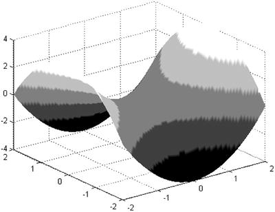
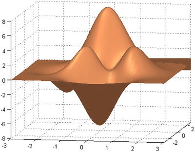
You can use some or all of these steps to create your graphic. So let’s go through a few examples. As a first example we consider the surface z = x2 - y2 in [-2,2] x [- 2,2] and represent it with strong lighting, shading dense grayish colors (Figure 5-25).
>> [X, and] = meshgrid(-2:0.05:2);
Z = X .^ 2 – Y .^ 2;
surf(X,Y,Z),shading interp,brighten(0.75),colormap(gray(5))
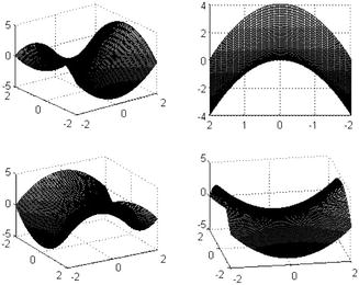
Then we represent, on the same axes, the curve focused from four different points of view and with shading by default (Figure 5-26).
>> [X, Y] = meshgrid(-2:0.05:2);
Z = X .^ 2 – Y .^ 2;
subplot(2,2,1)
surf(X,Y,Z)
subplot(2,2,2)
surf(X,Y,Z),view(-90,0)
subplot(2,2,3)
surf(X,Y,Z),view(60,30)
subplot(2,2,4)
surf(X,Y,Z),view(-10,30)
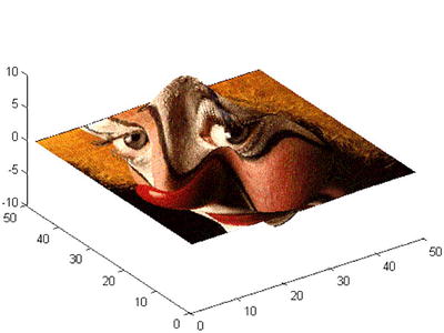
Then MATLAB reads a file and appropriate properties are used to generate the colorful graph in Figure 5-27.
>> load clown
surface(peaks,flipud(X),...
'FaceColor','texturemap',...
'EdgeColor','none',...
'CDataMapping','direct')
colormap(map)
view(-35, 45)
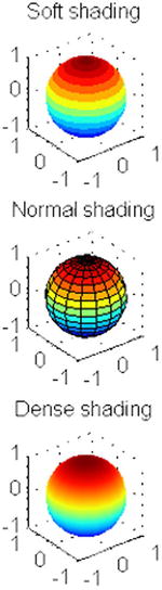
Our clown could use a ball, so let’s create one for him. Different shaders are used for the sphere (Figure 5-28).
>> subplot(3,1,1)
sphere(16)
axis square
shading flat
title('Soft shading')

subplot(3,1,2)
sphere(16)
axis square
shading faceted
title(' Normal shading')

subplot(3,1,3)
sphere(16)
axis square
shading interp
title('Dense shading')
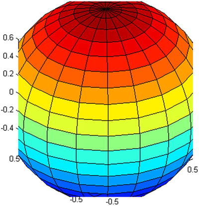
The following example changes the ratio of appearance for the sphere (Figure 5-29).
>> sphere
set(gca,'DataAspectRatio',[1 1 1],...
'PlotBoxAspectRatio',[1 1 1],'ZLim',[-0.6 0.6])

Now place the background color of the current figure in white (Figure 5-30).
>> set(gcf, 'Color', 'w')
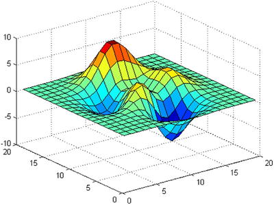
In the following example (Figure 5-31), we represent a surface utilizing the function peaks predefined in MATLAB (similar to a two-dimensional Gaussian distribution) with change of origin and scale.
>> surf(peaks(20))
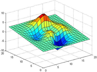
Then we rotate the figure above 180 degrees around the axis X (Figure 5-32).
>> h = surf(peaks(20));
rotate(h,[1 0 0],15)
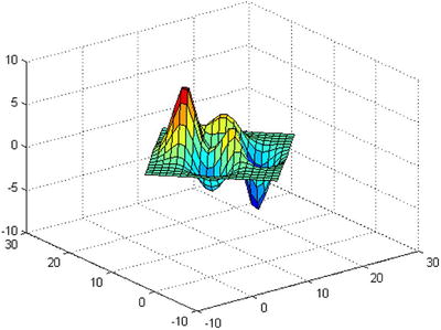
Then we change the center and rotate the start surface 45° in the direction of the axis z (Figure 5-33).
>> h = surf(peaks(20));
zdir = [0 0 1];
center = [10 10 0];
rotate(h,zdir,45,center)
In the following example we define several axes in a simple window (Figure 5-34).
>> axes('position',[.1  .1  .8  .6])
mesh(peaks(20));
axes('position',[.1  .7  .8  .2])
pcolor([1:10;1:10]);
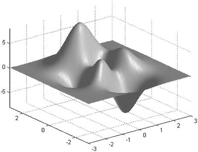
Then we equip special lighting, grey dense shading and variation of axes in [- 3, 3] x [- 3, 3] x [- 8, 8] to the peaks surface (Figure 5-35).
>> [x, y] = meshgrid(-3:1/8:3);
z = peaks(x,y);
surfl(x,y,z);
shading interp
colormap (gray);
axis([-3 3,-3 3,-8 8])
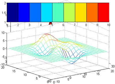
Then we change perspective, mesh and color to the previous illuminated surface (Figure 5-36).
>> view([10 10])
grid on
hold on
surfl(peaks)
shading interp
colormap copper
hold off
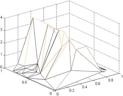
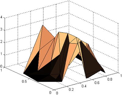
Below are two examples of triangle graphics (Figures 5-37 and 5-38). Note that because the rand function is used, your results will not be the same as these.
>> x = rand(1,50);
y = rand(1,50);
z = peaks(6*x-3,6*x-3);
tri = delaunay(x,y);
trimesh(tri,x,y,z)

>> x = rand(1,50);
y = rand(1,50);
z = peaks(6*x-3,6*x-3);
tri = delaunay(x,y);
trisurf(tri,x,y,z);
colormap copper
As you can see from the examples in this chapter, you have many options at your disposal to enhance or modify your graphics to suit your needs.