Problem

You need to make a numerical model of an air turbine to demonstrate detection filters.

Solution

Write the equations of motion for an air turbine. You will use a linear model of the air turbine to simplify the model and the detection filter design. This will allow you to model the system with a state space model.

How It Works

Figure 9-1 shows an air turbine.¹ It has a constant pressure air supply. You can control the valve from the air supply, the pressure regulator, to control the speed of the turbine. The air flows past the turbine blades causing it to turn. The control needs to adjust the air pressure to handle variations in the load. You measure the air pressure p downstream from the valve and you also measure the rotational speed of the turbine ω with a tachometer.

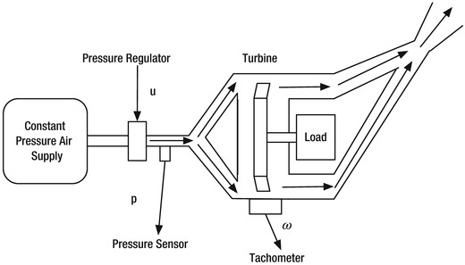
Figure 9-1. Air turbine. The arrows show the airflow. The air flows through the turbine blade tips, causing it to turn

The dynamical model for the air turbine is (9.1)

This is a state space system (9.2)
where (9.3)
(9.4)

The state vector is (9.5)

The pressure downstream from the regulator is equal to K _p u when the system is in equilibrium. τ _p is the regulator time constant and τ _t is the turbine time constant. The turbine speed is K _t p when the system is in equilibrium. The tachometer measures ω and the pressure sensor measures p. The load is folded into the time constant for the turbine.

The code for the right-hand side of the dynamical equations is shown next. Only one line of code is the right-hand side. The rest returns the default data structure. The simplicity of the model is due to its being a state space model. The number of states could be large, yet the code would not change.

function xDot = RHSAirTurbine( ˜, x, d )

% Default data structure

if ( nargin < 1 )

kP = 1;

kT = 2;

tauP = 10;

tauT = 40;

c = eye (2);

b = [kP/tauP;0];

a = [-1/tauP 0; kT/tauT -1/tauT];

xDot = struct('a',a,'b',b,'c',c,'u',0);

return

end

% Derivative

xDot = d.a*x + d.b*d.u;

The response to a step input for u is shown in Figure 9-2. The pressure settles faster than the turbine. This is due to the turbine time constant and the lag in the pressure change. The residuals are very small because there are no failures.

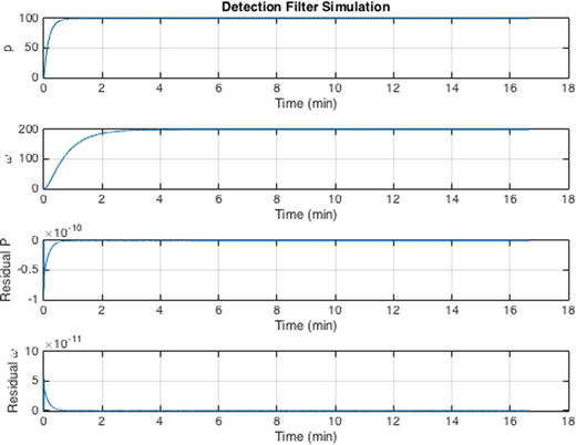
Figure 9-2. Air turbine response to a step pressure regulator input

Problem

You want to build a system to detect failures in an air turbine using the linear model developed in the previous recipe.

Solution

You will build a detection filter that detects pressure regulator failures and tachometer failures. Our plant model (continuous a, b, and c state space matrices) will be an input to the filter building function.

How It Works

The detection filter is an estimator with a specific gain matrix that multiplies the residuals. (9.6)
where is the estimated pressure and is the estimated angular rate of the turbine. The D matrix is the matrix of detection filter gains. These feed back the residuals, the difference between the measured and estimated states, into the detection filter. The residual vector is
(9.7)

The D matrix needs to be selected so that this vector tells you the nature of the failure. The gains should be selected so that

• The filter is stable.

• If the pressure regulator fails, the first residual, is non-zero but the second remains zero.

• If the turbine fails, the second residual is non-zero but the first remains zero.

The gain matrix is (9.8)

The time constant τ ₁ is the pressure residual time constant. The time constant τ ₂ is the tachometer residual time constant. In effect, you cancel out the dynamics of the plant and replace them with decoupled detection filter dynamics. These time constants should be shorter than the time constants in the dynamical model so that you detect failures quickly. However, they need to be at least twice as long as the sampling period to prevent numerical instabilities.

Write a function with three actions: an initialize case, an update case, and a reset case. varargin is used to allow the three cases to have different input lists. The function signature is

function d = DetectionFilter( action, varargin )

The header and syntax for DetectionFilter are shown next. Some LaTeX equations are used to describe the function.

%% DetectionFilter Builds and updates a linear detection filter .

% The detection filter gain matrix d is designed during the initialize

% action. The continuous matrices are then discretized using the internal

% function CToDZOH. The esimated state and residual vectors are initialized

% to the size dictated by a. During the update action, the residuals and

% new estimated state are calculated and stored in the data structure d .

%

% The residuals calculation is

%

% $$r = y - chat{x}$$

%

% The estimated state calculated with the detection filter gains is

%

% $$hat{x}_{k+1} = a*hat{x} + +b*u + d*r$$

%

%% Form:

% d = DetectionFilter( ' initialize ' , d, tau, dT );

% d = DetectionFilter( ' update ' , u, y, d );

% d = DetectionFilter( ' reset ' , d );

%

%% Inputs

% action (1,:) ' initialize ' or ' update '

% d (.) Data structure

% . a (:,:) State space continuous a matrix

% .b (:,1) State space continuous b matrix

% .c (:,:) State space continuous c matrix

% tau (:,1) Vector of time constants

% dT (1,1) Time step

% u (:,1) Actuation input

% y (:,1) Measurement vector

%

%% Outputs

% d (.) Updated data structure

% .a (:,:) State space discrete a matrix

% .b (:,1) State space discrete b matrix

% .c (:,:) State space discrete c matrix

% .d (:,:) Detection filter gain matrix

% .x (:,1) Estimated states

% .r (:,1) Residual vector

The filter is built and initialized in the following code in DetectionFilter. The continuous state space model of the plant, in this case our linear air turbine model, is an input. The selected time constants τ are also an input, and they are added to the plant model, as in equation 9.8. The function discretizes the plant a and b matrices and the computed detection filter gain matrix d.

switch lower (action)

case 'initialize'

d = varargin {1};

tau = varargin {2};

dT = varargin {3};

% Design the detection filter

d.d = d.a + diag (1./tau);

% Discretize both

d.d = CToDZOH( d.d, d.b, dT );

[d.a, d.b] = CToDZOH( d.a, d.b, dT );

% Initialize the state

m = size (d.a,1);

d.x = zeros (m,1);

d.r = zeros (m,1);

The update for the detection filter is in the same function. Note the equations are implemented as described in the header.

case 'update'

u = varargin {1};

y = varargin {2};

d = varargin {3};

r = y - d.c*d.x;

d.x = d.a*d.x + +d.b*u + d.d*r;

d.r = r;

Finally, create a reset action to allow you to reset the residual and state values for the filter in between simulations.

case 'reset'

d = varargin {1};

m = size (d.a,1);

d.x = zeros (m,1);

d.r = zeros (m,1);

end

Problem

You want to simulate a failure in the plant and demonstrate the performance of the failure detection.

Solution

You will build a MATLAB script that designs the detection filter using the function from the previous recipe and then simulates it with a user selectable pressure regulator or tachometer failure. The failure can be total or partial.

How It Works

The script designs a detection filter using DetectionFilter from the previous recipe and implements it in a loop. Runge-Kutta integration propagates the continuous domain right-hand-side of the air turbine, RHSAirTurbine. The detection filter is discrete time.

The script has two scale factors, uF and tachF, that multiply the regulator input and the tachometer output to simulate failures. Setting a scale factor to zero is a total failure and setting it to one indicates that the device is working perfectly. If you fail one, expect the associated residual to be non-zero and the other to stay at zero.

%% Simulation of a detection filter

% Simulates detecting failures of an air turbine.

% An air turbine has a constant pressure air source that sends air

% through a duct that drives the turbine blades. The turbine is

% attached to a load.

%

% The air turbine model is linear. Failures are modeled by multiplying

% the regulator input and tachometer output by a constant. A constant

% of 0 is a total failure and 1 is perfect operation.

%% User inputs

% Failures. Set to any number. 0 is total failure. 1 is working.

% uF scales the actuation u. tachF scales the rate measurement.

uF = 1;

tachF = 0;

% Time constants for failure detection

tau1 = 0.3; % sec

tau2 = 0.3; % sec

% End time

tEnd = 1000; % sec

% State space system

d = RHSAirTurbine;

%% Initialization

dT = 0.02; % sec

n = ceil (tEnd/dT);

% Initial state

x = [0;0];

%% Detection Filter design

dF = DetectionFilter('initialize',d,[tau1;tau2],dT);

%% Run the simulation

% Control. This is the regulator input.

u = 100;

% Plotting array

xP = zeros (4,n);

t = (0:n-1)*dT;

for k = 1:n

% Measurement vector including measurement failure

y = [x(1);tachF*x(2)]; % Sensor failure

xP(:,k) = [x;dF.r];

% Update the detection filter

dF = DetectionFilter('update',u,y,dF);

% Integrate one step

d.u = uF*u; % Actuator failure

x = RungeKutta( @RHSAirTurbine, t(k), x, dT, d );

end

%% Plot the states and residuals

[t,tL] = TimeLabel(t);

yL = {'p' 'omega' 'Residual P' 'Residual⊔omega' };

tTL = 'Detection⊔Filter⊔Simulation';

PlotSet( t, xP,'x⊔label',tL,'y⊔label',yL,'plot⊔title',tTL,'figure⊔title',tTL)

In Figure 9-3, the regulator fails and its residual is non-zero. In Figure 9-4, the tachometer fails and its residual is non-zero. The residuals show what has failed clearly. Simple boolean logic (i.e., if end statements) are all that is needed.

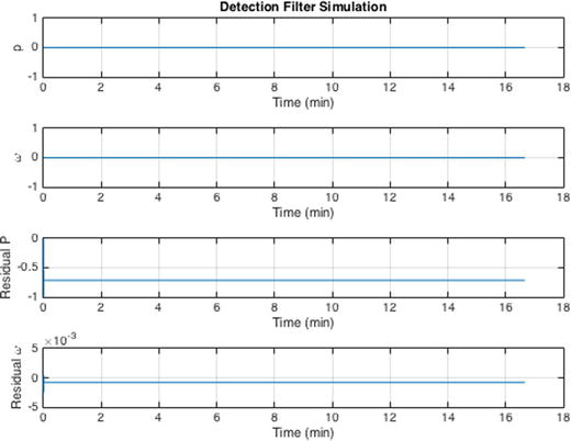
Figure 9-3. Air turbine response to a failed regulator

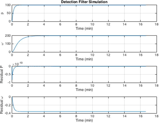
Figure 9-4. Air turbine response to a failed tachometer

Problem

You want a GUI to provide a graphical interface to the fault detection simulation that will allow you to evaluate the filter’s performance.

Solution

You will use the MATLAB GUIDE to build a GUI that allows you to

• Set the residual time constants.

• Set the end time for the simulation.

• Set the pressure regulator input.

• Introduce a pressure regulator or tachometer fault at any time.

• Display the states and residuals in a plot.

How It Works

The MATLAB GUI building system, GUIDE, is invoked by typing guide at the command line. There are several options for GUI templates, or a blank GUI; you will start from the GUI with uicontrols. First, let’s make a list of the controls you will need from our desired features list:

• Edit boxes for the simulation duration, residual time constants τ ₁ and τ ₂, pressure regulator setting u

• Edit boxes for the pressure regulator and tachometer fault parameters, with buttons for sending the newly commanded values to the simulation

• Text box for displaying the calculated detection filter gains

• Run button for starting a simulation

• Plot axes

In order to change the fault parameters while the simulation is running, you will need the loop to check a variable that can be externally set by the GUI. You can do this using global variables.

The template for the GUI controls gives you a couple edit boxes with labels, a set of radio buttons, and two action buttons for Calculate and Reset. You will use the edit boxes for the first two items on the list of controls and use the space with the radio buttons for the fault parameters. Figure 9-5 shows the template GUI in GUIDE before you make any changes to it.

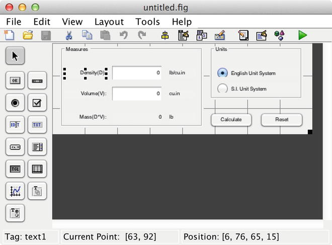
Figure 9-5. Template of a GUI with uicontrols

Simply double-click an item in the template GUI in GUIDE to open the inspector and edit the item’s text and font size, and so forth. For a text item, change the String field in the item’s Inspector. For a frame item, such as the Measures frame, change the Title field. For an edit box, change the Tag field. Make the following changes to the left-hand set of controls:

1. Change the String for the Density(D) label to “Duration”.

2. Change the String for the Volume(V) label to “Input”.

3. Increase the label font sizes to 10 pt.

4. Change the Tag for the density edit box to “duration”.

5. Change the Tag for the volume edit box to “input”.

6. Change the Tag for the mass text box to “gains”.

7. Change the Title of the Measures frame to “Parameters”.

After making these changes, click the green triangle button to save and run the GUI. MATLAB saves the .fig file with the name you specify, as well as a corresponding .m file. We choose to name our GUI DetectionFilterGUI. The resulting initial GUI is shown in Figure 9-6.

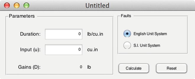
Figure 9-6. Snapshot of the GUI after the first few changes

At this point, you can start work on the GUI code itself. The template GUI stores its data, calculated from the data the user types into the edit boxes, in a field called metricdata. You can do a find/replace to change this field to filterdata throughout the m-file. Similarly, you can replace “density” with “duration” and “volume” with “input”. Changing the Tag of the edit boxes changes the name of the callback functions (i.e., from density_Callback to duration_Callback), but not the names of the variables inside the function bodies. The find/replace step is shown in Figure 9-7.

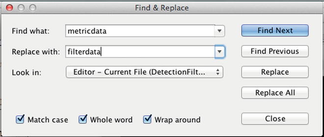
Figure 9-7. Find/Replace of metricdata fieldname

The updated duration_Callback function is shown next. You can keep the error-checking code that ensures that the input is a legitimate number. Note that MATLAB provides a nice hint on the best way to convert the contents of the graphics object from a string to a double, or how to keep it as a string. The guidata function stores the new value of the changed parameter in the figure itself using graphics handles.

function duration_Callback(hObject, eventdata, handles)

% hObject handle to duration (see GCBO)

% eventdata reserved – to be defined in a future version of MATLAB

% handles structure with handles and user data (see GUIDATA)

% Hints: get(hObject, ' String ' ) returns contents of duration as text

% str2double(get(hObject, ' String ' )) returns contents of duration as a double

duration = str2double( get (hObject, 'String'));

if isnan (filterdata)

set (hObject, 'String', 0);

errordlg('Input⊔must⊔be⊔a⊔number','Error');

end

% Save the new duration value

handles.filterdata.duration = duration;

guidata(hObject,handles)

The callback strings that are stored with the uicontrols can be seen in the Inspector by double-clicking the control, as shown in Figure 9-8, for the “duration” edit box.

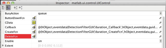
Figure 9-8. Callback strings for a uicontrol

The units, on the right-hand side of the edit boxes in the GUI, are being controlled by a function called by the units radio buttons. First, remove the entire Units panel; if you try to run the GUI now, it will throw an error due to the missing fields for the English and metric units. Next, remove the code relating to this “unitgroup” in the GUI’s m-file. You can also remove the code that sets the units fields, since you can hard-code these strings; in the template, they are labelled “text4”, “text5”, and “text6”. Remove lines in initialize_gui and the entire unitgroup_SelectionChangedFcn function.

Remove in initialize_gui():

set (handles.unitgroup, 'SelectedObject', handles.english);

set (handles.text4, 'String', 'lb/cu.in');

set (handles.text5, 'String', 'cu.in');

set (handles.text6, 'String', 'lb');

Set the initial values of the “duration” and inputs variables to the values from the simulation script:

handles.filterdata.duration = 1000;

handles.filterdata.input = 100;

Now, the GUI can run. You can change the units strings for the Duration, Input, and Gains in the Inspector now that you can removed the function that was setting them. You can give the figure a new name, Detection Filter GUI (click the figure background instead of one of the controls).

The next step is to add a new panel to the right-hand side of the GUI with edit boxes and buttons for failure parameters uF and tachF. Each items needs a Static Text uicontrol, the edit box, and a push button. The frame with these items added is shown in Figure 9-9.

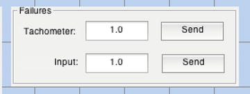
Figure 9-9. A panel with edit box and button uicontrols

Then, you can make the GUI and the panel on the right bigger; insert boxes for the time constants, τ ₁ and τ ₂; and add two plot axes. You have to leave a lot of room on the left-hand side of the axes for the axis labels. Change the Tag of the top axis to states and the bottom axis to residuals. The final GUI with all its uicontrols is shown in GUIDE in Figure 9-10. Note that the tags are shown on the axes.

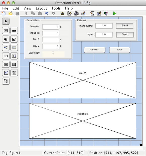
Figure 9-10. Finished GUI shown in GUIDE

Now, you have quite a bit of code to add to the GUI. The detection filter simulation goes in the Calculate callback. You have to add the code to convert the new edit box items to doubles, namely, tachF, uF, tau1, and tau2, as in the duration_Callback. You need to add code to the initialize_gui function to set values of all the fields. Finally, you need to add handling of global variables for the Send buttons on the failure parameters.

First, let’s make sure that the initialize function defines all the needed variables and then fix the edit box callbacks. You define the two global variables that you need for the failures.

% ---------------------------------------------------------

function initialize_gui(fig_handle, handles, isreset)

global tachFSent

global inputFSent

% If the filterdata field is present and the reset flag is false, it means

% we are we are just re-initializing a GUI by calling it from the cmd line

% while it is up. So, bail out as we dont want to reset the data.

if isfield (handles, 'filterdata') && ˜isreset

return ;

end

handles.filterdata.duration = 1000;

handles.filterdata. input = 100;

handles.filterdata.tau1 = 0.3;

handles.filterdata.tau2 = 0.3;

handles.filterdata.tachF = 1.0;

handles.filterdata.uF = 1.0;

handles.filterdata.dT = 0.1; % sec

handles.filterdata.dF = [];

set (handles.duration, 'String', handles.filterdata.duration);

set (handles. input, 'String', handles.filterdata. input);

set (handles.tau1, 'String', handles.filterdata.tau1);

set (handles.tau2, 'String', handles.filterdata.tau2);

set (handles.uF, 'String', handles.filterdata.uF);

set (handles.tachF, 'String', handles.filterdata.tachF);

set (handles.gains, 'String', '[]');

tachFSent = false;

inputFSent = false;

% Update handles structure

guidata (handles.figure1, handles);

UpdateGains(handles.figure1, [], handles);

The reset feature is from the template GUI; you will leave it because it allows a user to return to nominal values for all the fields if they get the filter into an unstable state. Note that you are adding a field for dT here and a variable dF, which stores the detection filter data structure. You add a call to a function UpdateGains after setting the GUI data in the handles; this function updates the stored detection filter when the fields for tau1 or tau2 are changed. This allows you to display them in the gains text box and avoid recomputing the filter matrices every time you do a simulation. You use num2str to display the gains matrix, with a maximum of digits of precision so that the matrix fits in the allotted space. The UpdateGains function is shown here.

function UpdateGains(hObject, eventdata, handles)

tau1 = handles.filterdata.tau1;

tau2 = handles.filterdata.tau2;

dT = handles.filterdata.dT;

d = RHSAirTurbine;

dF = DetectionFilter('initialize',d,[tau1;tau2],dT);

handles.filterdata.dF = dF;

set (handles.gains, 'String', num2str (dF.d,3));

guidata (hObject,handles)

Now you can update the callbacks for tau1 and tau2. After setting the value in the handles, you call the new update function, just as you did in the initialize function. The function for tau1 is shown next; the same changes must be made to tau2.

function tau1_Callback(hObject, eventdata, handles)

% hObject handle to tau1 (see GCBO)

% eventdata reserved - to be defined in a future version of MATLAB

% handles structure with handles and user data (see GUIDATA)

tau1 = str2double(get (hObject, 'String'));

if isnan (tau1)

set (hObject, 'String', 0);

errordlg ('Input⊔must⊔be a⊔number','Error');

end

% Save the new duration value

handles.filterdata.tau1 = tau1;

guidata (hObject,handles)

UpdateGains(hObject,[],handles);

Now, you need to set the Send button callbacks to set the global variables. The Send button tags were set to sendTach and sendInput, respectively. The only code needed in the callbacks is to declare and set the global variables to true. The function for sendInput is shown next; the same changes must be made to sendTach, using the tachFSent global variable.

% --- Executes on button press in sendInput.

function sendInput_Callback(hObject, eventdata, handles)

% hObject handle to sendInput (see GCBO)

% eventdata reserved 2013 to be defined in a future version of MATLAB

% handles structure with handles and user data (see GUIDATA)

global inputFSent

inputFSent = true;

Now, you are ready to add the Calculate function. It is based on the simulation script from the previous recipe. You add handling of the global variables to change the failure parameters during the simulation loop. You also add real-time plot updates to give the user immediate feedback on the residuals. The TimeLabel function is used to get the scale factor for the time labeling using the duration field, before the simulation loop starts.

You calculate a parameter, dP, for the number of steps between plotting by using floor. Basically, you update the plot 100 times during the simulation. In the loop, you plot dots for the current state, and residuals if the remainder of the current step k divided by dP is zero. Updating graphics using drawnow or by selecting axes in a loop can be very slow, so this is a simple method to limit the time spent on the graphics.

Also note that you use the form of plot where the axes handle can be passed in to avoid making the axes current using axes. MATLAB warns you that doing so can be very slow. However, there is no reason not to do so once the loop is finished, when creating the legends.

% --- Executes on button press in calculate.

function calculate_Callback(hObject, eventdata, handles)

% hObject handle to calculate (see GCBO)

% eventdata reserved – to be defined in a future version of MATLAB

% handles structure with handles and user data (see GUIDATA)

global inputFSent

global tachFSent

% get the data from the handles

u = handles.filterdata.input ;

duration = handles.filterdata.duration;

tachF = handles.filterdata.tachF;

uF = handles.filterdata.uF;

dT = handles.filterdata.dT;

% initialize the simulation states and arrays

n = ceil (duration/dT);

x = [0;0];

d = RHSAirTurbine;

dF = handles.filterdata.dF;

dF = DetectionFilter('reset',dF);

xP = zeros (4,n);

t = (0:n-1)*dT;

dP = floor (n/100);

% prepare for plotting during the simulation

[tt,tL] = TimeLabel(duration);

tF = tt/duration;

axes (handles.states)

cla

hold on

axes (handles.residuals)

cla

hold on

xlabel (tL)

for k = 1:n

if inputFSent

inputFSent = false;

data = guidata(hObject);

uF = data.filterdata.uF;

end

if tachFSent

tachFSent = false;

data = guidata(hObject);

tachF = data.filterdata.tachF;

end

y = [x(1);tachF*x(2)]; % Sensor failure

xP(:,k) = [x;dF.r];

dF = DetectionFilter('update',u,y,dF);

d.u = uF*u; % Actuator failure

x = RungeKutta( @RHSAirTurbine, t(k), x, dT, d );

if rem (k,dP)==0

plot (handles.states,tF*t(k), xP(1,k),'b.' );

plot (handles.states,tF*t(k), xP(2,k),'r.' );

plot (handles.residuals,tF*t(k), xP(3,k), 'b.' );

plot (handles.residuals,tF*t(k), xP(4,k), 'r.' );

drawnow

end

end

% Plot the states and residuals

axes (handles.states)

plot (tF*t, xP(1:2,:) )

legend ('p','omega')

axes (handles.residuals)

plot (tF*t, xP(3:4,:) )

legend ('r_p','r_{omega}')

Now, you have a functioning GUI that plots the progress of the simulation and allow you to inject faults at any time. Figure 9-11 shows the result of a simulation with no faults.

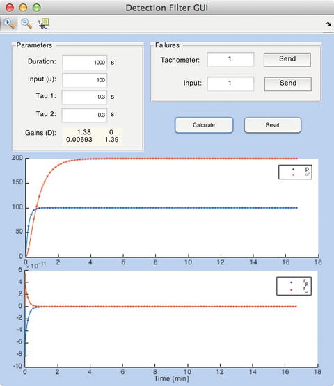
Figure 9-11. GUI runs with no faults

You have now built a tool that can be used to explore the parameter space of a model without generating dozens of plot windows. Note that adding a few toolbar buttons to enables the user to zoom or get data points from the plots. Additional features that could be added include menu items, such as saving and reloading particular cases, or exporting a run to the workspace, a mat-file, or a text file. Figure 9-12 shows a run with an input fault injected partway through the simulation. This affects the states as well as the residual. In order to replicate such a run, you would have to record the values of tachF and uF over time along with the initial conditions.

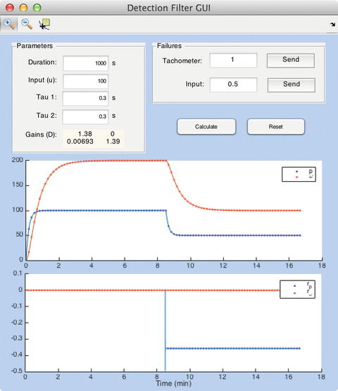
Figure 9-12. GUI run with injected input fault