Chapter 3: Your Data Science Workbench

In this chapter, you will learn about MLflow in the context of creating a local environment so that you can develop your machine learning project locally with the different features provided by MLflow. This chapter is focused on machine learning engineering, and one of the most important roles of a machine learning engineer is to build up an environment where model developers and practitioners can be efficient. We will also demonstrate a hands-on example of how we can use workbenches to accomplish specific tasks.

Specifically, we will look at the following topics in this chapter: 

• Understanding the value of a data science workbench
• Creating your own data science workbench
• Using the workbench for stock prediction

Technical requirements 

For this chapter, you will need the following prerequisites: 

• The latest version of Docker installed on your machine. If you don’t already have it installed, please follow the instructions at https://docs.docker.com/get-docker/.

  The latest version of Docker Compose installed. If you don’t already have it installed, please follow the instructions at https://docs.docker.com/compose/install/.

• Access to Git in the command line, and installed as described in this Uniform Resource Locator (URL): https://git-scm.com/book/en/v2/Getting-Started-Installing-Git.
• Access to a bash terminal (Linux or Windows). 
• Access to a browser.
• Python 3.5+ installed.
• MLflow installed locally, as described in Chapter 1, Introducing MLflow.

Understanding the value of a data science workbench

A data science workbench is an environment to standardize the machine learning tools and practices of an organization, allowing for rapid onboarding and development of models and analytics. One critical machine learning engineering function is to support data science practitioners with tools that empower and accelerate their day-to-day activities.

In a data science team, the ability to rapidly test multiple approaches and techniques is paramount. Every day, new libraries and open source tools are created. It is common for a project to need more than a dozen libraries in order to test a new type of model. These multitudes of libraries, if not collated correctly, might cause bugs or incompatibilities in the model.

Data is at the center of a data science workflow. Having clean datasets available for developing and evaluating models is critical. With an abundance of huge datasets, specialized big data tooling is necessary to process the data. Data can appear in multiple formats and velocities for analysis or experimentation, and can be available in multiple formats and mediums. It can be available through files, the cloud, or REpresentational State Transfer (REST) application programming interfaces (APIs).

Data science is mostly a collaborative craft; it’s part of a workflow to share models and processes among team members. Invariably, one pain point that emerges from that activity is the cross-reproducibility of model development jobs among practitioners. Data scientist A shares a training script of a model that assumes version 2.6 of a library, but data scientist B is using version 2.8 environment. Tracing and fixing the issue can take hours in some cases. If this problem occurs in a production environment, it can become extremely costly to the company.

When iterating—for instance—over a model, each run contains multiple parameters that can be tweaked to improve it. Maintaining traceability of which parameter yielded a specific performance metric—such as accuracy, for instance—can be problematic if we don’t store details of the experiment in a structured manner. Going back to a specific batch of settings that produced a better model may be impossible if we only keep the latest settings during the model development phase.

The need to iterate quickly can cause many frustrations when translating prototype code to a production environment, where it can be executed in a reliable manner. For instance, if you are developing a new trading model in a Windows machine with easy access to graphics processing units (GPUs) for inference, your engineering team member may decide to reuse the existing Linux infrastructure without GPU access. This leads to a situation where your production algorithm ends up taking 5 hours and locally runs in 30 seconds, impacting the final outcome of the project.

It is clear that a data science department risks systemic technical pain if issues related to the environment and tools are not addressed upfront. To summarize, we can list the following main points as described in this section:

• Reproducibility friction
• The complexity of handling large and varied datasets
• Poor management of experiment settings
• Drift between local and production environments

A data science workbench addresses the pain points described in this section by creating a structured environment where a machine learning practitioner can be empowered to develop and deploy their models reliably, with reduced friction. A no-friction environment will allow highly costly model development hours to be focused on developing and iterating models, rather than on solving tooling and data technical issues.

After having delved into the motivation for building a data science workbench for a machine learning team, we will next start designing the data science workbench based on known pain points.

Creating your own data science workbench

In order to address common frictions for developing models in data science, as described in the previous section, we need to provide data scientists and practitioners with a standardized environment in which they can develop and manage their work. A data science workbench should allow you to quick-start a project, and the availability of an environment with a set of starting tools and frameworks allows data scientists to rapidly jump-start a project.

The data scientist and machine learning practitioner are at the center of the workbench: they should have a reliable platform that allows them to develop and add value to the organization, with their models at their fingertips.

The following diagram depicts the core features of a data science workbench:

Figure 3.1 – Core features of a data science workbench

In order to think about the design of our data science workbench and based on the diagram in Figure 3.1, we need the following core features in our data science workbench:

• Dependency Management: Having dependency management built into your local environment helps in handling reproducibility issues and preventing library conflicts between different environments. This is generally achieved by using environment managers such as Docker or having environment management frameworks available in your programming language. MLflow provides this through the support of Docker- or Conda-based environments.
• Data Management: Managing data in a local environment can be complex and daunting if you have to handle huge datasets. Having a standardized definition of how you handle data in your local projects allows others to freely collaborate on your projects and understand the structures available.
• Model Management: Having the different models organized and properly stored provides an easy structure to be able to work through many ideas at the same time and persist the ones that have potential. MLflow helps support this through the model format abstraction and Model Registry component to manage models.
• Deployment: Having a development environment aligned with the production environment where the model will be serviced requires deliberation in the local environment. The production environment needs to be ready to receive a model from a model developer, with the least possible friction. This smooth deployment workflow is only possible if the local environment is engineered correctly.
• Experimentation Management: Tweaking parameters is the most common thing that a machine learning practitioner does. Being able to keep abreast of the different versions and specific parameters can quickly become cumbersome for the model developer.

  Important note

  In this section, we will implement the foundations of a data science workbench from scratch with MLflow, with support primarily for local development. There are a couple of very opinionated and feature-rich options provided by cloud providers such as Amazon Web Services (AWS) Sagemaker, Google AI, and Azure Machine Learning (Azure ML).

Machine learning engineering teams have freedom in terms of the use cases and technologies that the team they are serving will use.

The following steps demonstrate a good workflow for development with a data science workbench:

• The model developer installs the company workbench package through an installer or by cloning the repository.
• The model developer runs a command to start a project.
• The model developer chooses a set of options based on configuration or a prompt.
• The basic scaffolding is produced with specific folders for the following items:

  a) Data: This will contain all the data assets of your current project

  b) Notebooks: To hold all the iterative development notebooks with all the steps required to produce the model

  c) Model: A folder that contains the binary model or a reference to models, potentially in binary format

  d) Source Code: A folder to store the structured code component of the code and reusable libraries

  e) Output: A folder for any specific outputs of the project—for instance, visualizations, reports, or predictions

• A project folder is created with the standards for the organization around packages, dependency management, and tools.
• The model developer is free to iterate and create models using supported tooling at an organizational level.

Establishing a data science workbench provides a tool for acceleration and democratization of machine learning in the organization, due to standardization and efficient adoption of machine learning best practices.

We will start our workbench implementation in our chapter with sensible components used industrywide.

Building our workbench

We will have the following components in the architecture of our development environment:

• Docker/Docker Compose: Docker will be used to handle each of the main component dependencies of the architecture, and Docker Compose will be used as a coordinator between different containers of software pieces. The advantage of having each component of the workbench architecture in Docker is that neither element’s libraries will conflict with the other.
• JupyterLab: The de facto environment to develop data science code and analytics in the context of machine learning.
• MLflow: MLflow is at the cornerstone of the workbench, providing facilities for experiment tracking, model management, registry, and deployment interface.
• PostgreSQL database: The PostgreSQL database is part of the architecture at this stage, as the storage layer for MLflow for backend metadata. Other relational databases could be used as the MLflow backend for metadata, but we will use PostgreSQL.

Our data science workbench design can be seen in the following diagram:

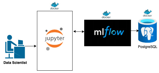
Figure 3.2 – Our data science workbench design

Figure 3.2 illustrates the layout of the proposed components that will underpin our data science workbench.

The usual workflow of the practitioner, once the environment is up and running, is to develop their code in Jupyter and run their experiments with MLflow support. The environment will automatically route to the right MLflow installation configured to the correct backend, as shown in Figure 3.2.

Important note

Our data science workbench, as defined in this chapter, is a complete local environment. As the book progresses, we will introduce cloud-based environments and link our workbench to shared resources.

A sample layout of the project is available in the following GitHub folder:

https://github.com/PacktPublishing/Machine-Learning-Engineering-with-MLflow/tree/master/Chapter03/gradflow

You can see a representation of the general layout of the workbench in terms of files here:

├── Makefile

├── README.md

├── data

├── docker

├── docker-compose.yml

├── docs

├── notebooks

├── requirements.txt

├── setup.py

├── src

├── tests

└── tox.ini

The main elements of this folder structure are outlined here:

• Makefile: This allows control of your workbench. By issuing commands, you can ask your workbench to set up a new environment notebook to start MLflow in different formats.
• README.md: A file that contains a sample description of your project and how to run it.
• data folder: A folder where we store the datasets used during development and mount the data directories of the database when running locally.
• docker: A folder that encloses the Docker images of the different subsystems that our environment consists of.
• docker-compose.yml: A file that contains the orchestration of different services in our workbench environment—namely: Jupyter Notebooks, MLflow, and PostgreSQL to back MLflow.
• docs: Contains relevant project documentation that we want persisted for the project.
• notebooks: A folder that contains the notebook information.
• requirements.txt: A requirements file to add libraries to the project.
• src: A folder that encloses the source code of the project, to be updated in further phases of the project.
• tests: A folder that contains end-to-end testing for the code of the project.
• tox.ini: A templated file that controls the execution of unit tests.

We will now move on to using our own development environment for a stock-prediction problem, based on the framework we have just built.

Using the workbench for stock prediction

In this section, we will use the workbench step by step to set up a new project. Follow the instructions step by step to start up your environment and use the workbench for the stock-prediction project.

Important note

It is critical that all packages/libraries listed in the Technical requirements section are correctly installed on your local machine to enable you to follow along.

Starting up your environment

We will move on next to exploring your own development environment, based on the development environment shown in this section. Please execute the following steps:

1. Copy the contents of the project available in https://github.com/PacktPublishing/Machine-Learning-Engineering-with-MLflow/tree/master/Chapter03/gradflow.
2. Start your local environment by running the following command:

   make

3. Inspect the created environments, like this:

   $ docker ps

   The following screenshot presents three Docker images: the first for Jupyter, the second for MLflow, and the third for the PostgreSQL database. The status should show Up x minutes:

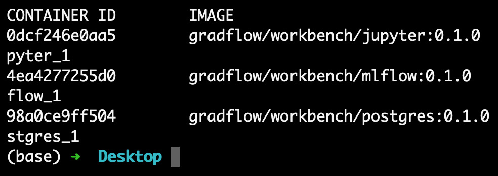
Figure 3.3 – Running Docker images

The usual ports used by your workbench are listed as follows: Jupyter serves in port 8888, MLflow serves in port 5000, and PostgreSQL serves in port 5432.

In case any of the containers fail, you might want to check if the ports are used by different services. If this is the case, you will need to turn off all of the other services.

Check your Jupyter Notebooks environment at http://localhost:8888, as illustrated in the following screenshot:

Figure 3.4 – Running Jupyter environment

You should have a usable environment, allowing you to create new notebooks file in the specified folder.

Check your MLflow environment at http://localhost:5000, as illustrated in the following screenshot:

Figure 3.5 – Running MLflow environment

Figure 3.5 shows your experiment tracker environment in MLflow that you will use to visualize your experiments running in MLflow.

Run a sample experiment in MLflow by running the notebook file available in /notebooks/mlflow_sample.ipynb, as illustrated in the following screenshot:

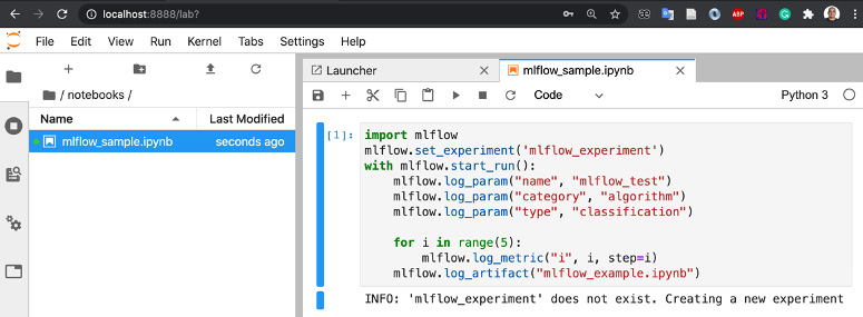
Figure 3.6 – Excerpt of mlflow_sample code

The code in Figure 3.6 imports MLflow and creates a dummy experiment manually, on the second line, using mlflow.set_experiment(‘mlflow_experiment’).

The with mlflow.start_run() line is responsible for starting and tearing down the experiment in MLflow.

In the three following lines, we log a couple of string-type test parameters, using the mlflow.log_param function. To log numeric values, we will use the mlflow.log_metric function.

Finally, we also log the entire file that executed the function to ensure traceability of the model and code that originated it, using the mlflow.log_artifact(“mlflow_example.ipynb”) function.

Check the sample runs, to confirm that the environment is working correctly. You should go back to the MLflow user interface (UI) available at http://localhost:5000 and check if the new experiment was created, as shown in the following screenshot:

Figure 3.7 – MLflow test experiment

Figure 3.7 displays the additional parameters that we used on our specific experiment and the specific metric named i that is visible in the Metrics column.

Next, you should click on the experiment created to have access to the details of the run we have executed so far. This is illustrated in the following screenshot:

Figure 3.8 – MLflow experiment details

Apart from details of the metrics, you also have access to the mlflow_example notebook file at a specific point in time.

At this stage, you have your environment running and working as expected. Next, we will update it with our own algorithm; we’ll use the one we created in Chapter 2, Your Machine Learning Project.

Updating with your own algorithms

Let’s update the notebook file that we created in Chapter 2, ML Problem Framing, and add it to the notebook folder on your local workbench. The code excerpt is presented here:

import mlflow

class RandomPredictor(mlflow.pyfunc.PythonModel):

  def __init__(self):

    pass

  def predict(self, context, model_input):

    return model_input.apply(lambda column: random.randint(0,1))

Under the notebook folder in the notebooks/stockpred_randomizer.ipynb file, you can follow along with the integration of the preceding code excerpt in our recently created data science workbench. We will proceed as follows:

1. We will first import all the dependencies needed and run the first cell of the notebook, as follows:
   

   Figure 3.9 – MLflow experiment details

2. Let’s declare and execute the class outlined in Figure 3.9, represented in the second cell of the notebook, as follows:
   

   Figure 3.10 – Notebook cell with the RandomPredictor class declaration

3. We can now save our model in the MLflow infrastructure so that we can test the loading of the model. model_path holds the folder name where the model will be saved. You need to instantiate the model in an r variable and use mlflow.pyfunc.save_model to save the model locally, as illustrated in the following code snippet:
   

   Figure 3.11 – Notebook demonstrating saving the model

   You can see on the left pane of your notebook environment that a new folder was created alongside your files to store your models. This folder will store the Conda environment and the pickled/binarized Python function of your model, as illustrated in the following screenshot:

   

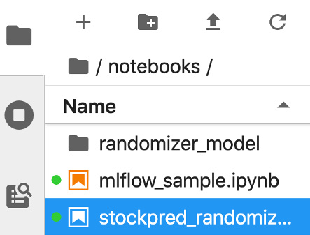
   Figure 3.12 – Notebook demonstrating the saved model folder

4. Next, we can load and use the model to check that the saved model is usable, as follows:

Figure 3.13 – Notebook demonstrating the saved model folder

Figure 3.14 demonstrates the creation of a random input pandas DataFrame and the use of loaded_model to predict over the input vector. We will run the experiment with the name stockpred_experiment_days_up, logging as a metric the number of days on which the market was up on each of the models, as follows:

Figure 3.14 – Notebook cell demonstrating use of the loaded model

To check the last runs of the experiment, you can look at http://localhost:5000 and check that the new experiment was created, as illustrated in the following screenshot:

Figure 3.15 – Initial UI of MLflow for our stockpred experiment

You can now compare multiple runs of our algorithm and see differences in the Days Up metric, as illustrated in the following screenshot. You can choose accordingly to delve deeper on a run that you would like to have more details about:

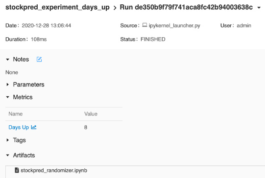
Figure 3.16 – Logged details of the artifacts saved

In Figure 3.16, you can clearly see the logged details of our run—namely, the artifact model and the Days Up metric.

In order to tear down the environment properly, you must run the following command in the same folder:

make down

Summary

In this chapter, we introduced the concept of a data science workbench and explored some of the motivation behind adopting this tool as a way to accelerate our machine learning engineering practice.

We designed a data science workbench, using MLflow and adjacent technologies based on our requirements. We detailed the steps to set up your development environment with MLflow and illustrated how to use it with existing code. In later sections, we explored the workbench and added to it our stock-trading algorithm developed in the last chapter.

In the next chapter, we will focus on experimentation to improve our models with MLflow, using the workbench developed in this chapter.

Further reading

In order to further your knowledge, you can consult the documentation in the following links: 

• Cookiecutter documentation page: https://cookiecutter.readthedocs.io/en/1.7.2/
• Reference information about cookie cutters: https://drivendata.github.io/cookiecutter-data-science/
• The motivation behind data science workbenches: https://dzone.com/articles/what-is-a-data-science-workbench-and-why-do-data-s#