Model performance is a broad term generally used to measure how the model performs on a new dataset, usually a test dataset. The performance metrics also play the role of thresholds to decide whether the model can be put into actual decision making systems or needs improvements. In the previous chapter, we discussed some performance metrics for our continuous and discrete cases. In this chapter, we will discuss how changing the modeling process can help us improve model performance on the metrics.
Feature selection plays an important role in modeling development process. It is the features that have information to explain the dependent variable. Data scientists spend a lot of time selecting and creating features for fitting predictive models. The feature engineering process involves selection of a best set of features and their transformations. These sets of features are then fed into a algorithm to quantify the relationships. The algorithm learns from the data and creates a predictive model. The performance of such a model is then evaluated based on some kind of error measure. Model performance improvement methods are then applied to boost the performance on the error metrics of interest. The higher levels properties of a model, e.g., complexity and speed of learning, also impact the model performance. These high-level parameters are known as hyper-parameters. We will discuss hyper-parameters more in the following sections. Broadly there are two ways to improve the model performance, specifically in machine learning algorithms:
Add more features and improve the quality of data
Optimize the hyper-parameters
This first point is what we have been discussing so far in the book. However, we also discussed some algorithms where the learning process is influenced by hyper-parameters, e.g., in decision trees, the depth of the tree, the number of folds in cross validation, etc. Now these parameters are independent of the features and influence the model performance. For instance, you can have two different decision tree models using the same set of predictors but different hyper-parameters to train them. To understand the performance optimization process, we need to understand the trade of between bias and variance. Bias refers to the difference between the true and predicted values, while variance refers to the spread around the mean of predicted values. Bias and variance are the two vital components of imprecision/performance in predictive models, and in general there is a tradeoff between them. The tradeoff is nonlinear, which means normally reducing one leads to increasing the other.
This chapter will look at these issues and provide illustrations in R to equip you on how to implement some of the popular performance improvement techniques using R.
The content of this chapter is oriented toward broader awareness of the latest developments in the computational world due to increased computational power and business acceptance of concepts. The dataset for this chapter is the same as the previous chapter (purchase prediction and house sale price), as we show you how the concepts from this chapter influence the results from previous metrics.
Note
The R illustrations in this chapter are computationally heavy, so you are advised to check the machine configuration before running these examples.
While we try to balance out simplicity and completeness in this chapter, we expect the user of these techniques to have good understanding of numerical computing and the machine learning algorithm. References to research papers will be shared for detailed reading on statistical underpinnings.
Learning objectives for this chapter:
Machine learning and statistical modeling
Overview of Caret package
Introduction to hyper-parameters
Hyper-parameter tuning illustrations
Bias versus variance tradeoffs
Introduction to ensemble learning
Advanced methods in ensemble learning
Advanced topic: Bayesian optimization
8.1 Machine Learning and Statistical Modeling
The comparison of machine learning and statistical modeling has been a key debate topic in recent times. Machine learning has become a very popular term, and this is getting stronger as the computational power is increasing. In this section of chapter, we try to express the opinion based on some of the learning arguments in this debate. The core of this debate does not divide machine learning and statistics into two exclusive groups but it will make you more aware about how you can solve a problem with data.
At core of machine learning/statistical modeling is quantifying the relationship between the response variable and predictors. Mathematically, the relationship can be written as a function:
Y = f(X) + e
Where
f(): Function of X
X: An input vector with X1, X1.Xn.
Y: Output
E: The random error
The way we treat the estimation problem is what differentiates machine learning from statistical modeling. Machine learning is an algorithm that can learn this relationship without relying on any rule-bases programming. Statistical modeling will estimate the relationship based on formal quantification from statistical inferences (confidence interval, hypothesis testing, distributions, etc.). The process of statistical inference quantifies the process by which data is generated, while machine learning will emphasize how the final predictions will look if similar data is supplied in the future.
Statistical learning terminology also differs from machine learning, for instance we say estimation in statistics but learning in machine learning. There are other numerous cases where the terminology is different due to the fact that the origin of achieving same objective has been different. Here are a few more examples:
Classifier -> Hypothesis
Regression/Classification -> Supervised Learning
Clustering -> Unsupervised Learning
Robert Tibshirani, a statistician and machine learning expert at Stanford, says machine learning is a glamorous version of statistics. Although statistical analysis and methodology is the predominant approach in modern machine learning, not all machine learning methods are based on probabilistic models, e.g., SVMs and non-negative matrix factorization.
Machine learning is also computationally costly and needs more computing power, which helps in solving many complex problems. One more difference is the size of data normally in these two fields—statistics usually deals with low dimensional spaces while machine learning is used in higher dimensional space. When we have hundreds of features and millions of data points, so upholding statistical principles becomes impossible. In such situations, we employ techniques that are based on salable and less assumption learning methods.
The machine learning tools and techniques are capable of learning from trillions of observations one by one. They make predictions and learn simultaneously. Algorithms like random forest and gradient boosting are exceptionally robust and fast, with a wide variety (high dimension/features) and depth of features (a high number of observations). However, statistical modeling is generally applied for smaller datasets with fewer attributes or they end up overfitting. Also, these methods are spared from the assumptions that are required in statistical learning. Machine learning algorithms in general can be used with any distribution and/or with any boundary conditions to train a model.
The best analogy so far comes from nature and the way humans learn. We don’t learn things around us based on assumptions but learn from trials. Similarly, machine learning is an adaption of learning from multiple iterations, in which for each iteration we try to get close to the actual values. As the guiding principle for machine learning is to replicate a system, its predictive power is generally very strong. This helps in putting all the variables before knowing their relation to the response variable, so the algorithm takes care of any misfit variable. However, statistical models are mathematics-intensive and based on coefficient estimation. They require the modeler to understand the relationship between variables before putting it in.
In a nutshell, machine learning is not as deterministic as a statistical modeling. With the scope of learning, it becomes very important how we ask our machine algorithm to learn from data. We can actually influence the model performance by managing the rules of how the machine should learn. While for statistical models the options are limited to inputs and preset assumptions for the statistical method.
8.2 Overview of the Caret Package
The Caret package is one of the most powerful packages in R. This package allows users to explore the machine learning algorithms to their fullest potential. The Caret package (short for classification and regression training) contains functions for complex regression and classification problems . The package has a dedicated Git page and is one of the actively updated and documented packages of R. The Caret package is created and maintained by Max Kuhn from Pfizer.
The Caret package has a lot of dependencies on other R packages. The required packages are only loaded when required and hence save a lot of overhead time and computational power. For instance, randomForest library is loaded only if you use rf as one of the model methods. You can install this package with or without the dependencies. You can install it including all dependent 27 packages using the suggests field; otherwise Caret loads packages as needed and assumes that they are installed.
install.packages("caret", dependencies =c("Depends", "Suggests"))You are encouraged to visit the Caret project page and keep the updated information from there. The home page of the project is at http://caret.r-forge.r-project.org/ and the Git page can be accessed at http://topepo.github.io/caret/index.html .
The Caret package has numerous functions for model development and evaluation metrics for performance measurement. Being a comprehensive package it can be used for other techniques in sampling and also for sophisticated feature selection processes. There are two of the most important function/tools in the Caret package:
trainControl()
train()
The trainControl() function is like a wrapper that defines the rule for model training and the conditions around how sampling and grid search is to be done. The train() function is very powerful function that can support 230 types of models available in the Caret package. The primary function/tool, train(), can be used for:
Model evaluation, using cross validation, resampling, and other conventional metrics. It also can be used to measure the effect of tuning parameters in performance.
Model selection by choosing the best model based on optimal parameters, so multiple metrics can be calculated to choose the final model.
Model estimation using any of the 230 types of models listed in the train model list with default parameters or tuned ones.
By default, the function automatically chooses the tuning parameters associated with the best value, although different algorithms can be used to tune the parameters (Source: http://topepo.github.io/caret/model-training-and-tuning.html ).

Figure 8-1. The train() function algorithm in the Caret package
In general, the basic use of the Caret package includes first defining trainControl()and then calling the train() function. Here we show the generic syntax of calling these two functions in order to use the Caret functionality.
Others are available, such as repeated K-fold cross validation, leave-one-out, etc. The function train control can be used to specify the type of resampling. By default, a simple bootstrap resampling is used:
rfControl <-trainControl(# Example, 10-fold Cross Validationmethod ="repeatedcv", # Others are available, such as repeated K-fold cross-validation, leave-one-out etcnumber =10, # Number of foldsrepeats =10# repeated ten times)
The first two arguments to train are the predictor and outcome data objects, respectively. The third argument, method, specifies the type of model (see train model list or train models by tag). Here is an example that fits a randomForest model via the randomForest package, which was tested with 10-fold cross validation:
set.seed(917)randomForectFit1 <-train(Class ∼., # Define the model equationdata = training, # Define the modeling datamethod ="rf", # List the model you want to use, caret provide list of options in train Model listtrControl = rfControl, # This defines the conditions on how to control the training... ) # Other options specific to the modeling techniquerandomForectFit1
More information about trainControl is given in a later section. Details can be found at http://topepo.github.io/caret/model-training-and-tuning.html .
As this is the core package in R, it deals with almost all of the machine learning techniques. Therefore, it’s important to keep in mind its functionality.
Note
In this chapter we will not be using the full dataset. The illustrations will be on smaller set of data to make sure you can replicate the results on less powerful machines.
8.3 Introduction to Hyper-Parameters
In machine learning, we deal with two kind of parameters, ones that are the standard model parameters and ones that are the hyper-parameters. The core difference between these two types of parameters is that model parameters can be directly learned from the underlying data and hyper-parameters cannot. The machine learning model training process is used to learn the data and then fit the model parameters.
However, the hyper-parameters are not directly learned from the data and are actually very influential in model performance. Hyper-parameters explain the "higher-level" properties of the model such as its complexity, how fast it should learn, and how much depth it should go into. Another important thing is that hyper-parameters are fixed before training starts, hence, the model standard parameters are learned. We can say that hyper-parameters decide the rules of model training by which model standard parameters are estimated.
Now, how are the hyper-parameter decided? What influences the hyper-parameter selection process? This area is summed up as hyper-parameter optimization and will be touched upon at a high level in an upcoming section.
The hyper-parameters differ from the standard model parameters (or coefficients). Some of the properties of hyper-parameter are listed here:
Explain higher level properties: Define the complexity of model, capacity to learn, optimization criteria, etc.
Not directly learned: They cannot be learned from underlying data, like the standard model parameters can. They are the property of machine learning algorithm and the learning space and need to be predefined.
Iterative optimization: They can be set at different values and then evaluated on model performance, so in the most primitive sense, they can be optimized by iteratively finding the value that tests better.
Another way to look at hyper-parameters is as a prerequisite for a Bayesian approach to statistical learning, which involves finding the probability distribution of the model parameters given a training dataset. For instance, an artificial network training will require four preset hyper-parameters for learning from the data: selection of the model type with algorithm, selection of the architecture of the network, assignment of training parameters, and learning the model parameters. Generally, we can divide the hyper-parameters into four decision points before we train the model with data:
Model type: Decide what type of model you choose in machine learning, like feed-forward or recurrent neural network, support vector machine, linear regression, etc.
Architecture: Once you decide the model type, you give inputs on what the boundaries of the model learning process are, i.e., number of hidden layers, number of nodes per hidden layer, batch normalization and pooling layer, etc.
Training-parameter: Once you decide on the model type and architecture, you decide how the model should learn, i.e., learning and momentum rate, batch size, etc. These parameters are sometimes called training parameter.
Model parameter: Once you provide these inputs, the model training process starts and the model parameters are estimated, such as weights and biases in a neural network.
Some examples of hyper-parameters are:
Depth of trees or number of leaves
Latent factors in a matrix factorization
Learning rate (in neural network based methods)
Hidden layers in a deep neural network
Number of clusters in a k-means clustering
To illustrate the effect of hyper-parameters on the model performance, we will create a example with different hyper-parameters and check the performance of the model. For this example, we will use a subset of the purchase prediction data.
In the following example, we are creating two random forest models with the same underlying data and the same predictor variables, but with two different values for the hyper-parameter (the number of trees):
ntree = 20
ntree = 50
Here are the accuracy results for both cases:
setwd("C:/Personal/Machine Learning/Run Chap 8");library(caret)library(randomForest)set.seed(917);# Load DatasetPurchase_Data <-read.csv("Purchase Prediction Dataset.csv",header=TRUE)#Remove the missing valuesdata <-na.omit(Purchase_Data)#Pick a sample of recordsData <-data[sample(nrow(data),size=10000),]
Model 1: with tree size = 20
Here are the results for the algorithm using 20 trees in the random forest algorithm.
fit_20 <-randomForest(factor(ProductChoice) ∼MembershipPoints +CustomerAge +PurchaseTenure +CustomerPropensity +LastPurchaseDuration,data=Data,importance=TRUE,ntree=20)#Print the result for ntree=20print(fit_20)
Here are the results for the algorithm using 20 trees in the random forest algorithm .
Call:randomForest(formula = factor(ProductChoice) ∼ MembershipPoints + CustomerAge + PurchaseTenure + CustomerPropensity + LastPurchaseDuration, data = Data, importance = TRUE, ntree = 20)Type of random forest: classificationNumber of trees: 20No. of variables tried at each split: 2OOB estimate of error rate: 64.27%Confusion matrix:1 2 3 4 class.error1 550 1035 495 104 0.74816852 730 1927 1051 199 0.50678273 449 1300 1005 165 0.65570404 149 450 300 91 0.9080808
Model 1 with tree size = 50
Here are the results for the algorithm using 50 trees in the random forest algorithm.
fit_50 <-randomForest(factor(ProductChoice) ∼MembershipPoints +CustomerAge +PurchaseTenure +CustomerPropensity +LastPurchaseDuration,data=Data,importance=TRUE,ntree=50)#Print the result for ntree=50print(fit_50)Call:randomForest(formula = factor(ProductChoice) ∼ MembershipPoints + CustomerAge + PurchaseTenure + CustomerPropensity + LastPurchaseDuration, data = Data, importance = TRUE, ntree = 50)Type of random forest: classificationNumber of trees: 50No. of variables tried at each split: 2OOB estimate of error rate: 63.35%Confusion matrix:1 2 3 4 class.error1 502 1153 472 57 0.77014652 712 2065 994 136 0.47146153 427 1329 1029 134 0.64748204 147 467 307 69 0.9303030
We can see by just changing the hyper-parameters that the results are different. The overall error rate in ntree=50 has come down to 63.35% from 64.27%. Among the classification in each class, the classification rate of classes 1 and 4 improved by approx. 3% while from classes 2 and 3, it decreased. Now the next important question to answer is what is the most cost- and time-effective way to find an optimal value of the hyper-parameters.
8.4 Hyper-Parameter Optimization
In machine learning, hyper-parameter optimization or model selection is the process of choosing a set of hyper-parameters for a machine learning algorithm. The set of hyper-parameters that maximize the model performance are then chosen for actual model training and testing. Cross validation is generally used for measuring the performance of the model in terms of cross validation error rate or some other user-defined method, e.g., bootstrap error, leave-one-out, etc.
In short, learning algorithms learn model parameters that model/fit the input data well, while hyper-parameter optimization is to ensure the model does not overfit its data by tuning, e.g., regularization. There are multiple algorithms suggested to optimize the hyper-parameters of any algorithm. There are multiple popular packages and paid services also available to optimize the parameters. Most of them are based on some or another variation of the Bayesian approach. We will illustrate the parameter tuning by different methods on the same model. This will help you get a comparative understanding of how the results change and what can be influencing them.
The most popular methods are listed here, with some context. We are not providing any direct comparison of these methods as the selection of method is influenced by many factors, including but not limited to type of model, computation power, time-space complexity, etc.
Manual search: Create a set of parameters using best judgment/experience and test them on the model. Choose the one that works best for the model performance.
Manual grid search: Create an equally spaced grid or custom grid of a combination of hyper-parameters. Evaluate the mode on each grid point and choose the ones with the best model performance.
Automatic grid search: Let the program decide a grid for you and do the search in that space for the best hyper-parameters,
Optimal search: In this method we generally don’t freeze the grid beforehand, but allow the machine to expand the grid as and when needed.
Random search: In general, choosing some random points in the hyper-parameter search space works faster and better. Although this saves lot of spatial and time cost, it might not always give you the best/optimal set of hyper-parameters.
Custom search: Users can define their own functions and guide the algorithm on how to find the best set of hyper-parameters.
Note
Most of these parameter tuning/optimization techniques are search problems in high dimensional space. The searching is done on a iterative and guided basis, mostly numerical only. The following sections illustrate the popular optimization methods.
8.4.1 Manual Search
The details of the model for manual search optimization are discussed in this section.
Response Variable: ProductChoice
Predictors: MembershipPoints, CustomerAge, PurchaseTenure, CustomerPropensity, and LastPurchaseDuration
Error Calculation: Cross Validation
Model Type: Random Forest
# Manually search parameterslibrary(data.table)# load the packageslibrary(randomForest)library(mlbench)library(caret)# Load Datasetdataset <-Datametric <- "Accuracy"
Here, we set the trainControl function with the method=”repeatedCV”, meaning use repeated cross validation, and search method = “grid”, meaning search in the grid defined by tunegrid.
# Manual SearchtrainControl <-trainControl(method="repeatedcv", number=10, repeats=3, search="grid")tunegrid <-expand.grid(.mtry=c(sqrt(ncol(dataset)-2)))modellist <-list()
Here, we set the train function with method=”rf”, meaning use the random forest algorithm to fit the model and number of trees as ntree from the loop variables.
for (ntree in c(100, 150, 200, 250)) {set.seed(917);fit <-train(factor(ProductChoice) ∼MembershipPoints +CustomerAge +PurchaseTenure +CustomerPropensity +LastPurchaseDuration, data=dataset, method="rf", metric=metric, tuneGrid=tunegrid, trControl=trainControl, ntree=ntree)key <-toString(ntree)modellist[[key]] <-fit}# compare results by resamplingresults <-resamples(modellist)#Summary of Resultssummary(results)Call:summary.resamples(object = results)Models: 100, 150, 200, 250Number of resamples: 30AccuracyMin. 1st Qu. Median Mean 3rd Qu. Max. NA’s100 0.3880 0.3990 0.4107 0.4081 0.4134 0.4364 0150 0.3890 0.3996 0.4117 0.4094 0.4147 0.4390 0200 0.3864 0.3974 0.4095 0.4081 0.4139 0.4360 0250 0.3884 0.4013 0.4097 0.4090 0.4167 0.4390 0KappaMin. 1st Qu. Median Mean 3rd Qu. Max. NA’s100 0.04385 0.06549 0.08044 0.07803 0.08661 0.1209 0150 0.05301 0.06481 0.08014 0.07977 0.08831 0.1235 0200 0.04243 0.06214 0.07847 0.07757 0.08953 0.1196 0250 0.04427 0.06311 0.08145 0.07873 0.08884 0.1244 0#Dot Plot of resultsdotplot(results)

Figure 8-2. Performance plot accuracy metrics
You can see the accuracy doesn’t vary much between the different parameter values. This can mean that our search is not comprehensive or the model is able to learn most of the features of data in less than the 100-tree random forest model. Also, the independent variables list should be increased.
8.4.2 Manual Grid Search
The details of the model for manual grid search optimization are discussed in this section.
Response Variable: ProductChoice
Predictors: MembershipPoints, CustomerAge, PurchaseTenure, CustomerPropensity, and LastPurchaseDuration
Error Calculation: Cross Validation
Model Type:Learning Vector Quantization (LVQ)
# Tune algorithm parameters using a manual grid search.seed <-917;dataset <-Data
Here, we set the trainControl function with method=”repeatedCV”, meaning use repeated cross validation, and the search method = “grid”, meaning search in the grid defined by grid.
# prepare training schemecontrol <-trainControl(method="repeatedcv", number=10, repeats=3)# design the parameter tuning gridgrid <-expand.grid(size=c(5,10,20,50), k=c(1,2,3,4,5))# train the modelmodel <-train(factor(ProductChoice) ∼MembershipPoints +CustomerAge +PurchaseTenure +CustomerPropensity +LastPurchaseDuration, data=dataset, method="lvq", trControl=control, tuneGrid=grid)# summarize the modelprint(model)Learning Vector Quantization10000 samples5 predictor4 classes: ’1’, ’2’, ’3’, ’4’No pre-processingResampling: Cross-Validated (10 fold, repeated 3 times)Summary of sample sizes: 9001, 9000, 9000, 9001, 8999, 9000, ...Resampling results across tuning parameters:size k Accuracy Kappa5 1 0.3403649 0.015088575 2 0.3443983 0.024647505 3 0.3582986 0.031185535 4 0.3556306 0.029338875 5 0.3510002 0.0334276610 1 0.3375292 0.0279086310 2 0.3387723 0.0302415210 3 0.3398577 0.0301609610 4 0.3484939 0.0403084710 5 0.3457038 0.0474341520 1 0.3403710 0.0401305720 2 0.3321322 0.0295645920 3 0.3380415 0.0393496320 4 0.3422641 0.0421395220 5 0.3449026 0.0461146650 1 0.3353654 0.0358839450 2 0.3358704 0.0325533150 3 0.3428662 0.0436931050 4 0.3421693 0.0471398050 5 0.3437377 0.04756819Accuracy was used to select the optimal model using the largest value.The final values used for the model were size = 5 and k = 3.# plot the effect of parameters on accuracyplot(model)
The tuning algorithm shows the best tuning parameters Figure 8-3 also shows the top line peaking on the accuracy plot, which correspond to the best model.

Figure 8-3. Accuracy across cross-validated samples
8.4.3 Automatic Grid Search
The details of the model for automatic grid search optimization are discussed in this section.
Response Variable: ProductChoice
Predictors: MembershipPoints, CustomerAge, PurchaseTenure, CustomerPropensity, and LastPurchaseDuration
Error Calculation: Cross Validation
Model Type:Learning Vector Quantization (LVQ)
# Tune algorithm parameters using an automatic grid search.set.seed(917);dataset <-Data
Here, we set the trainControl function with method=”repeatedCV”, meaning use repeated cross validation and the search method being default, i.e., an automatic grid search.
# prepare training schemecontrol <-trainControl(method="repeatedcv", number=10, repeats=3)# train the modelmodel <-train(factor(ProductChoice) ∼MembershipPoints +CustomerAge +PurchaseTenure +CustomerPropensity +LastPurchaseDuration, data=dataset, method="lvq", trControl=control, tuneLength=5)# summarize the modelprint(model)Learning Vector Quantization10000 samples5 predictor4 classes: ’1’, ’2’, ’3’, ’4’No pre-processingResampling: Cross-Validated (10 fold, repeated 3 times)Summary of sample sizes: 9000, 8999, 9001, 9001, 9000, 9000, ...Resampling results across tuning parameters:size k Accuracy Kappa11 1 0.3402322 0.0366663511 6 0.3402335 0.0351844711 11 0.3394009 0.0409331011 16 0.3499678 0.0441570711 21 0.3444298 0.0420899013 1 0.3379881 0.0352333713 6 0.3459702 0.0482657113 11 0.3464008 0.0501049713 16 0.3467346 0.0505507213 21 0.3497683 0.0560035816 1 0.3313684 0.0381365716 6 0.3460655 0.0501351816 11 0.3417672 0.0464688716 16 0.3502685 0.0497727716 21 0.3456003 0.0475558519 1 0.3299696 0.0322951019 6 0.3392352 0.0457655519 11 0.3361026 0.0385975419 16 0.3479016 0.0506701519 21 0.3451598 0.0499700022 1 0.3365661 0.0345459622 6 0.3459982 0.0439915422 11 0.3441293 0.0459216322 16 0.3506335 0.0518767922 21 0.3512329 0.05437707Accuracy was used to select the optimal model using the largest value.The final values used for the model were size = 22 and k = 21.# plot the effect of parameters on accuracyplot(model)

Figure 8-4. Accuracy across cross validated samples for an automatic grid search
The automatic grid search optimization shows the best model would be with parameters of size=22 and k= 21, which corresponds to an accuracy of 0.3512. This differs from our manual grid search, where the optimal parameters were size= 5 and k=3, with an accuracy of 0.3581.
8.4.4 Optimal Search
The details of the model for optimal search optimization are discussed in this section.
Response Variable: ProductChoice
Predictors: MembershipPoints, CustomerAge, PurchaseTenure, CustomerPropensity, and LastPurchaseDuration
Error Calculation: Cross Validation
Model Type:Recursive PartitioningandRegression Trees
Observe the following three expand.grids we used for the tuneGrid parameter in the train function.
Manual search: expand.grid(.mtry=c(sqrt(ncol(dataset)-2)))
Manual grid search: expand.grid(size=c(5,10,20,50), k=c(1,2,3,4,5))
Optimal search: expand.grid(.cp=seq(0,0.1,by=0.01))
In the optimal search, the parameters to expand.grid are more granular, which means the algorithm will be able to converge to a global optimum much better than the others. For example, by modifying the by = 0.01 in the seq function to have more decimal places, you can further increase the granularity. However, keep in mind that increasing the granularity will take computational effort.
# Select the best tuning configurationdataset <-Data
Here, we set the trainControl function with the method=”repeatedCV”, meaning use repeated cross validation, and parameter tuning is done on tunegrid.
# prepare training schemecontrol <-trainControl(method="repeatedcv", number=10, repeats=3)# CARTset.seed(917);tunegrid <-expand.grid(.cp=seq(0,0.1,by=0.01))fit.cart <-train(factor(ProductChoice) ∼MembershipPoints +CustomerAge +PurchaseTenure +CustomerPropensity +LastPurchaseDuration, data=dataset, method="rpart", metric="Accuracy", tuneGrid=tunegrid, trControl=control)Loading required package: rpartfit.cartCART10000 samples5 predictor4 classes: ’1’, ’2’, ’3’, ’4’No pre-processingResampling: Cross-Validated (10 fold, repeated 3 times)Summary of sample sizes: 9000, 8999, 9001, 9001, 9000, 9000, ...Resampling results across tuning parameters:cp Accuracy Kappa0.00 0.3557312 0.059431920.01 0.4014336 0.041792960.02 0.3966989 0.024817390.03 0.3907000 0.000000000.04 0.3907000 0.000000000.05 0.3907000 0.000000000.06 0.3907000 0.000000000.07 0.3907000 0.000000000.08 0.3907000 0.000000000.09 0.3907000 0.000000000.10 0.3907000 0.00000000Accuracy was used to select the optimal model using the largest value.The final value used for the model was cp = 0.01.# display the best configurationprint(fit.cart$bestTune)cp2 0.01plot(fit.cart)
The plot in Figure 8-5 clearly shows the peak of accuracy is at a cp value equal to 0.1, which corresponds to an accuracy of 0.41, which is higher than our previous optimized models. Also observe our model in this case is Recursive Partitioning and Regression Trees.
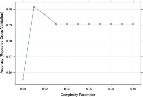
Figure 8-5. Accuracy across cross validated samples and complexity parameters
8.4.5 Random Search
The details of the model for random search optimization are discussed in this section.
Response Variable: ProductChoice
Predictors: MembershipPoints, CustomerAge, PurchaseTenure, CustomerPropensity, and LastPurchaseDuration
Error Calculation: Cross Validation
Model Type: Random Forest
# Randomly search algorithm parameters# Select the best tuning configurationdataset <-Data
Here, we set the trainControl function with method=”repeatedCV”, meaning use repeated cross validation, and the predictor search set to random.
# prepare training schemecontrol <-trainControl(method="repeatedcv", number=10, repeats=3, search="random")# train the modelmodel <-train(factor(ProductChoice) ∼MembershipPoints +CustomerAge +PurchaseTenure +CustomerPropensity +LastPurchaseDuration, data=dataset, method="rf", trControl=control)# summarize the modelprint(model)Random Forest10000 samples5 predictor4 classes: ’1’, ’2’, ’3’, ’4’No pre-processingResampling: Cross-Validated (10 fold, repeated 3 times)Summary of sample sizes: 9000, 9000, 9002, 9000, 9000, 8999, ...Resampling results across tuning parameters:mtry Accuracy Kappa3 0.4091006 0.077723324 0.3863345 0.080397526 0.3640687 0.06873901Accuracy was used to select the optimal model using the largest value.The final value used for the model was mtry = 3.# plot the effect of parameters on accuracyplot(model)

Figure 8-6. Accuracy across cross validated sets and randomly selected predictors
Random search algorithms are usually faster and more efficient in tuning. In this case, the plot shows that the algorithm was able to optimize the problem with fewer iterations. The random forest model is used in this example. Random forests are optimized quickly with random search. This saves lot of time in tuning random forest models.
8.4.6 Custom Searching
Custom search algorithms provide advanced ways of guiding the algorithm to optimize tuning parameters. Advanced users of machine learning can create their own search algorithms to optimize hyper-parameters. In this example, we show one such search optimization.
Response Variable: ProductChoice Predictors: MembershipPoints, CustomerAge, PurchaseTenure, CustomerPropensity and LastPurchaseDuration Error Calculation: Cross Validation Model Type: custom Random Forest
setwd("C:/Personal/Machine Learning/Chapter 8/");library(caret)library(randomForest)library(class)# Load DatasetPurchase_Data <-read.csv("Purchase Prediction Dataset.csv",header=TRUE)data <-na.omit(Purchase_Data)#Create a sample of 10K recordsset.seed(917);Data <-data[sample(nrow(data),size=10000),]# Select the best tuning configurationdataset <-Data# Customer Parameter Search# load the packageslibrary(randomForest)library(mlbench)library(caret)
In this example, we have come up with a custom function for evaluation. The algorithm of randomForest is inherited for a classification problem. This is an advanced way of creating your own search functions.
# define the custom caret algorithm (wrapper for Random Forest)customRF <-list(type="Classification", library="randomForest", loop=NULL)customRF$parameters <-data.frame(parameter=c("mtry", "ntree"), class=rep("numeric", 2), label=c("mtry", "ntree"))customRF$grid <-function(x, y, len=NULL, search="grid") {}customRF$fit <-function(x, y, wts, param, lev, last, weights, classProbs, ...) {randomForest(x, y, mtry=param$mtry, ntree=param$ntree, ...)}customRF$predict <-function(modelFit, newdata, preProc=NULL, submodels=NULL) { predict(modelFit, newdata)}customRF$prob <-function(modelFit, newdata, preProc=NULL, submodels=NULL) { predict(modelFit, newdata, type ="prob")}customRF$sort <-function(x){ x[order(x[,1]),]}customRF$levels <-function(x) {x$classes}# Load Datasetdataset <-Datametric <- "Accuracy"# train modeltrainControl <-trainControl(method="repeatedcv", number=10, repeats=3)tunegrid <-expand.grid(.mtry=c(1:4), .ntree=c(100, 150, 200, 250))set.seed(917)custom <-train(factor(ProductChoice) ∼MembershipPoints +CustomerAge +PurchaseTenure +CustomerPropensity +LastPurchaseDuration, data=dataset, method=customRF, metric=metric, tuneGrid=tunegrid, trControl=trainControl)print(custom)10000 samples5 predictor4 classes: ’1’, ’2’, ’3’, ’4’No pre-processingResampling: Cross-Validated (10 fold, repeated 3 times)Summary of sample sizes: 9000, 8999, 9001, 9001, 9000, 9000, ...Resampling results across tuning parameters:mtry ntree Accuracy Kappa1 100 0.4091336 0.050882261 150 0.4078343 0.049442091 200 0.4082998 0.049735711 250 0.4076663 0.048610502 100 0.4141003 0.072569692 150 0.4145340 0.073068972 200 0.4142334 0.072329832 250 0.4144336 0.072895163 100 0.4090333 0.079808043 150 0.4081328 0.077443573 200 0.4079661 0.077822253 250 0.4086323 0.078180174 100 0.3797990 0.072447854 150 0.3804304 0.072312284 200 0.3826303 0.075665504 250 0.3838646 0.07796204Accuracy was used to select the optimal model using the largest value.The final values used for the model were mtry = 2 and ntree = 150.plot(custom)

Figure 8-7. Accuracy across cross validated samples and parameter mtry
Custom search optimization gives us the highest accuracy of 0.415 so far. For this problem this seems to be the best accuracy. Again, to emphasize, we were using the same data and the same variable and saw how performance kept on varying. The next section will discuss a very important concept in model performance, bias, and variance.
8.5 The Bias and Variance Tradeoff
The errors in any machine learning algorithm can be attributed to bias, variance, and a irreducible error. The tradeoff or dilemma of bias and variance is the problem of minimizing bias and variance simultaneously in any machine learning algorithm. In general, reducing one tends to increase the other.
In performance measurement, we say bias causes underfitting, while variance causes overfitting. Figure 8-8 shows a very good graphical representation, provided by Scott Fortmann-Roe, in his blog using a bulls eye diagram.

Figure 8-8. Bias and variance Illustration using the bulls eye plot
Fortmann further provides a conceptual definition of errors due to bias and variance. Looking at the image in Figure 8-8, it becomes easy to visualize how errors due to bias and variance impact results. The simple definition is provided by Fortmann-Roe:
Error due to bias: The error due to bias is taken as the difference between the expected (or average) prediction of our model and the correct value that we are trying to predict.
Error due to variance: The error due to variance is taken as the variability of a model prediction for a given data point. Again, imagine that you can repeat the entire model building process multiple times. The variance is how much the predictions for a given point vary between different realizations of the model (Source: http://scott.fortmann-roe.com/docs/BiasVariance.html ).
The breaking of generalization errors in machine learning algorithms is called bias-variance decomposition , and it reduces the errors into three components :
Square of bias
Variance
Irreducibleerror
Mathematically, the decomposed equation looks like this:![]()
where![]()
and![]()
The derivation of this equation is also easy and can be done for generalized cases, as follows.
For any random variable
, variance is defined as![]()
Equivalently![]()
assume, ![]() and
and ![]() , as f is deterministic.
, as f is deterministic.![]()
Hence, ![]() and
and ![]() imply
imply![]()
Also, ![]()
Hence, ![]()
Since, ϵ and ![]() are independent, we have
are independent, we have

The irreducible error is the noise term in the true relationship that cannot fundamentally be reduced by any model. This derivation in the linear regression setup is explained in "Notes on Derivation of Bias-Variance Decomposition in Linear Regression," by Shakhnarovich, Greg (2011). A similar decomposition is possible in other machine learning algorithms.
Further, the tradeoff is shown here. The graphical representation of this tradeoff also gives us an idea as to how to tweak our machine learning algorithms to reach that sweet spot where the variance and bias are minimum given this tradeoff constraint.
The following code snippet shows this tradeoff on a real model prototype . In the following example, we calculate mean square error, bias, and variance for hypothetical data, and then plot how varying the value of shrink, a number vector, changes these quantities.
mu <-2Z <-rnorm(20000, mu)MSE <-function(estimate, mu) {return(sum((estimate -mu)^2) /length(estimate))}n <-100shrink <-seq(0,0.5, length=n)mse <-numeric(n)bias <-numeric(n)variance <-numeric(n)for (i in 1:n) {mse[i] <-MSE((1 -shrink[i]) *Z, mu)bias[i] <-mu *shrink[i]variance[i] <-(1 -shrink[i])^2}
Now let’s the plot the Bias-Variance tradeoff using the plot function ; we can use the ggplot function as well.
# Bias-Variance tradeoff plotplot(shrink, mse, xlab=’Shrinkage’, ylab=’MSE’, type=’l’, col=’pink’, lwd=3, lty=1, ylim=c(0,1.2))lines(shrink, bias^2, col=’green’, lwd=3, lty=2)lines(shrink, variance, col=’red’, lwd=3, lty=2)legend(0.02,0.6, c(’Bias^2’, ’Variance’, ’MSE’), col=c(’green’, ’red’, ’pink’), lwd=rep(3,3), lty=c(2,2,1))
You can see in the plot in Figure 8-9 that the variance and bias have the opposite behavior. The best optimal point for a model exists where the bias and variance meet. And this is the point that we try to use for the final model. The early indications of the model performance suffering from bias or variance can be seen by fitting the model on the test data. Test data is not seen by the model and hence we can measure its true performance or error on test data/hold out data.

Figure 8-9. Bias versus variance tradeoff plot
Model suffering from variance : When the model fits well on the train data but poorly fits on the test data. This shows that the variability of prediction is high and high variance error is dominating.
Model suffering from bias : When the model fits poorly on both train and test data. The error due to bias is driving the bad performance of the model.
Having a good understanding of the bias-variance tradeoff helps you decide which methods can be applied to correct for bias or variance issues in the model. But before we jump to the main methods of performance improvements by dealing with bias and variance, we list a few common steps that might be taken to improvement the model performance:
Bring more data into the model
Bring in more features
Revisit feature selection and create stronger features
Regularization methods of feature selection can help
Sampling can also be explored (upsample/downsample/resample)
Try other learning algorithms
Once you are satisfied with these steps, you can think of applying them to improve model performance.
8.5.1 Bagging or Bootstrap Aggregation
This can be used to train the same model on multiple samples, which reduces variance.
If the modeling is repeated n number of times, i.e., you create your model on n samples with each sample independent of the others, you get the variance by a factor of n. In other words, if you perform n replications of each configuration and let![]()
And since the Z_{j}s are independent of identically distributed random variables:
![$$ mathrm{V}mathrm{a}mathrm{r}left[Z(n)
ight]=frac{mathrm{Var}left[{Z}_j
ight]}{n}. $$](http://images-20200215.ebookreading.net/19/4/4/9781484223345/9781484223345__machine-learning-using__9781484223345__A416805_1_En_8_Chapter_Equi.gif)
This shows that developing models on multiple samples will reduce the bias. Monte Carlo methods have a detailed theory around this behavior of large sample statistics.
8.5.2 Boosting
Boosting successively models from errors, which reduces bias. Boosting repeatedly develops models on the residuals to get better accuracy. For example, the first model is developed and it gives 70% accuracy, then the 30% inaccurately predicted cases are used to develop another model to bring additional accuracy. This process is repeated until there is no improvement in accuracy. After infinite iterations, you are left with an irreducible error that contains no additional information.
We will discuss these methods in more detail after introducing the idea of ensemble learning. Ensemble learning is a method of using multiple models to solve a modeling problem. Ensemble learning is very effective in reducing the bias and variance of models. Another important aspect to keep in mind before we do a deep dive is the complexity of the model and production environment. As the model becomes more complex, it becomes difficult to interpret and implement in actual business applications. A data scientist has to be very careful in choosing the methods to reduce errors, as there is a cost-benefit analysis of the degree of improvement.
In general, we might not get into the decomposition of error, but mostly focus on the total error only. A set of data scientists believe that the incremental benefits are not that great compared to computational and complexity cost. Instead, we should focus on using an accurate measure of prediction error and explore different levels of model complexity and then choose the complexity level that minimizes the overall error.
8.6 Introduction to Ensemble Learning
The general idea of ensemble learning is better decision making with collective intelligence. The ensemble techniques are certainly a game changer in machine learning. In statistics and machine learning, ensemble learning means learning from multiple algorithms to improve the model performance .
Generally, the supervised algorithms perform the task of searching for a solution in hypothesis/parameter space and finding a suitable hypothesis/parameter that fits the problem at hand. As with any search problem, we can’t always find the best solution in limited iterations. In such situations, ensembles can be used to combine multiple hypotheses to form a (generally) better hypothesis.
As more than one model is involved in the process of ensemble, they are obviously computationally heavy as well as difficult to evaluate on a single parameter. In general, fast algorithms are recommended to be used in ensemble methods, e.g., decision tree ensembles (randomForest); however, slower algorithm benefit from ensemble methods equally. Similarly, you can apply ensemble learning to unsupervised learning algorithms. An ensemble learns from underlying models, hence it is itself a supervised learning algorithm .
We will use an example to understand the benefits of ensemble learning by "voting ensembles".
8.6.1 Voting Ensembles
Voting ensembles are the most popular ensemble method in classification problems. This ensemble combines the final class results from multiple models and chooses the one with the majority vote. It need not be only majority votes; you can weight them based on multiple other factors, e.g., individual model performance, complexity, etc. For explaining an example of an ensemble, Figure 8-10 is a illustration of majority votes.

Figure 8-10. Voting ensemble learning for a classification problem
(Source: Ensemble learning prediction of protein–protein interactions using proteins functional annotations by Saha,Zubek et.al.)
Now to help internalize the idea of voting ensembles, let’s understand from a hypothetical example, as illustrated here.
Problem: Finding defective bulbs (=1) in a manufactured lot of bulbs
Ensemble models: We have three inspection experts (read models) A, B, and C, to identify defective pieces. You can use any one of them or all of them.
Additional information: Accuracy of A is 0.7, accuracy of B is 0.6, and accuracy of C is 0.65. Their decision is independent of any other decision.
We have three binary classifiers models (A, B, and C) with 0.7, 0.6, and 0.65 accuracy, respectively. We will now show what happens if all of these models are used together in an ensemble model with the majority vote.
For a majority vote with three models, we can expect four outcomes:
All three are correct
0.7 * 0.68 * 0.65 = 0.3094
Two are correct
0.7 * 0.68 * 0.35
0.7 * 0.32 * 0.65
0.3 * 0.68 * 0.65 = 0.4448
Two are wrong
0.3 * 0.32 * 0.65
0.3 * 0.68 * 0.35
0.7 * 0.32 * 0.35 = 0.2122
All three are wrong
0.3 * 0.32 * 0.35 = 0.0336
In scenario 2, we can see that on average, the majority vote ensemble corrects for ∼44% of the cases. This ensemble of three models will give us an average accuracy of ∼75.4% (0.4448 + 0.3094), which is more than any individual model. However, the important consideration to see this kind of increase is the assumption that the models were independent of each other and their prediction was independent of each other. This independence condition generally doesn’t hold and hence sometimes you might struggle to see improvements in model performance, even with high dimensional ensemble.
8.6.2 Advanced Methods in Ensemble Learning
Broadly, there are two types of ensemble helping in variance and bias reduction. There are some variants around the same idea like blending, stacking, and custom ensembles, but the core idea can be explained by the two methods of bagging and boosting.
8.6.2.1 Bagging
Bootstrap aggregation, also called bagging, is a ensemble meta-algorithm. This algorithm improves the stability and accuracy of the model and reduces the overfitting issue. This method can be used with any method; in cases of continuous functions, it take weighed average the output of models, in classification, it weighs output to ensemble into one single output.
Bagging was proposed by Leo Breiman in 1994 for improving results of a classification problem. Details of his original work can be found in his technical paper, "Bagging Predictors" Technical Report No. 421, 1994, Department of Statistics.
Figure 8-11 shows a bagging ensemble flow. The steps in bagging are broadly divided into four parts:
Creating samples from training data; number of samples should be of appropriate numbers (not too many or too few).
Train the model on individual samples.
Create classifiers from each model and store the results.
Based on the type of ensemble, weighted or majority vote or some custom way. Combine the results to predict the test data.

Figure 8-11. Bagging ensemble flow
The image in Figure 8-11 illustrates the four steps in bagging mentioned earlier (Source: http://cse-w`iki.unl.edu/ ).
Consider these important features of bagging:
Each model is developed in parallel and independent of each other
Helps decrease the variance but ineffective in reducing bias
Best suited for high variance, low bias models (complex models)
RandomForest is a good example (the randomForest algorithm prunes the tree to reduce correlation)
8.6.2.2 Boosting
Similar to bagging, boosting is also a ensemble meta-algorithm meant to reduce bias in supervised learning models. Historically, boosting tries to answer the question, suppose we have a classifier that always gives a classification less than 50% (weak classifier). Can we build a sequence of models to reach zero error (minimal error)? Theoretically, this is possible by successively passing the residual to successive models. In general, the successive models create so many convoluted relationships in final models that it becomes difficult to explain the models; hence, boosting sometimes is known to create a black box, something very hard to explain and understand.
For instance, if you design three-pass boosting, and suppose the classifier is always 40% correct, then for a set of 100 objects in first pass we will have 60 misclassified. In the second pass, it only pass the misclassified objects, so 36% will be misclassified (60% of 60). Again in the third pass, you pass the misclassified and get 22% misclassified. So essentially, by using a classifier with only 40% accuracy, you can create a ensemble with an error equal to 22% (22/100) only, or a model with 78% accuracy.
However, in reality the theoretical underpinnings remain the same, but the improvements are not that dramatic, as many other factors come in to play, e.g., with each pass the model becomes weak, reweighing, correlation etc.
Figure 8-12 shows a boosting ensemble flow. The steps in boosting are described here:
First fit a model on a full training dataset, in Figure 8-12, you get 42% accuracy in the first model.
Fit another classifier and get 65% accuracy.
Fit the third model to get 92% accuracy.
Now you combine these different classifiers, to form a strong classifier.

Figure 8-12. Boosting ensemble flow
(Source: https://alliance.seas.upenn.edu ). You can see here that the boosted machine. i.e., the combined classifier, is performing far better than individual classifiers.
A few important features of boosting are listed here:
Each model is developed sequentially, so each successive model is built on the previous model-lacking area.
Helps decrease the bias, but is ineffective in reducing variance.
Best suited for low variance, high bias models.
Gradient boosting machine is a powerful algorithm using boosting ensemble.
In the following sections, we will show one example of each bagging, boosting, blending, and stacking on our purchase prediction data. The output tables are easy to read and the plot will make the process of model improvement clear.
Note that the parameters are not tuned for the examples.
8.7 Ensemble Techniques Illustration in R
Ensemble training is broadly of two types—bagging and boosting. However, there are many other variants researchers have proposed. In this section, we show some examples in R using our purchase prediction data.
This section shows a chunk of R codes, which are reproducible for any dataset you want to use. The specific function calls and their options can be accessed in the documentation of the Caret package and other dependencies.
For all of the following examples, there are three important functions to calibrate for each of the techniques:
trainControl(): Sets the sampling method, summary, and other training parameters.
train(): Trains the models with the trainControl() parameters; the modeling method is also defined in this function.
Ensemble method: Combines the results from different models using custom functions, resample, or caretEnsemble functions.
Let’s now start building ensemble models using the R environment.
8.7.1 Bagging Trees
The two most popular bagging algorithms are used here:
Bagged CART (regression tree)
Random forest
The following code creates two models based on these techniques and shows the comparison between these two tree methods.
library(caret)library(randomForest)library(class)library(ipred)# Load DatasetPurchase_Data <-read.csv("Purchase Prediction Dataset.csv",header=TRUE)data <-na.omit(Purchase_Data)# Create a sample of 10K recordsset.seed(917);Data <-data[sample(nrow(data),size=10000),]# Select the best tuning configurationdataset <-Data# Example of Bagging algorithmscontrol <-trainControl(method="repeatedcv", number=10, repeats=3)metric <- "Accuracy"
The following code snippet fits a bagged tree model.
# Bagged CARTset.seed(917)fit.treebag <-train(factor(ProductChoice) ∼MembershipPoints +CustomerAge +PurchaseTenure +CustomerPropensity +LastPurchaseDuration, data=dataset, method="treebag", metric=metric, trControl=control)Loading required package: plyrLoading required package: e1071
The following code snippet fits a Random Forest model.
# Random Forestset.seed(917)fit.rf <-train(factor(ProductChoice) ∼MembershipPoints +CustomerAge +PurchaseTenure +CustomerPropensity +LastPurchaseDuration, data=dataset, method="rf", metric=metric, trControl=control)
This summarizes the bagged results from the two methods using the resamples() function in the Caret package.
# summarize resultsbagging_results <-resamples(list(treebag=fit.treebag, rf=fit.rf))summary(bagging_results)Call:summary.resamples(object = bagging_results)Models: treebag, rfNumber of resamples: 30AccuracyMin. 1st Qu. Median Mean 3rd Qu. Max. NA’streebag 0.327 0.3444 0.3505 0.3518 0.3583 0.384 0rf 0.395 0.4095 0.4167 0.4151 0.4216 0.435 0KappaMin. 1st Qu. Median Mean 3rd Qu. Max. NA’streebag 0.02242 0.04812 0.05498 0.05786 0.06759 0.1044 0rf 0.04252 0.06536 0.07513 0.07387 0.08290 0.1032 0dotplot(bagging_results)
The accuracy for the random forest is better than the bagged CART. The plot in Figure 8-13 shows the comparison of both algorithms on Kappa and accuracy.

Figure 8-13. Accuracy and Kappa of bagged tree
8.7.2 Gradient Boosting with a Decision Tree
For boosting, we will see the two most popular algorithms:
C5.0: Decision tree developed by Ross Quinlan
Gradient Boosting Machine
The following code first creates a C5.0 decision tree model and then a GBM model . Once we have both models ready, we create a boosting ensemble with these two models combined.
library(C50)library(gbm)dataset <-Data;# Example of Boosting Algorithmscontrol <-trainControl(method="repeatedcv", number=10, repeats=3)metric <- "Accuracy"
Here, we are fitting a C5.0 decision tree model.
# C5.0set.seed(917)fit.c50 <-train(factor(ProductChoice) ∼MembershipPoints +CustomerAge +PurchaseTenure +CustomerPropensity +LastPurchaseDuration, data=dataset, method="C5.0", metric=metric, trControl=control)fit.c50C5.010000 samples5 predictor4 classes: ’1’, ’2’, ’3’, ’4’No pre-processingResampling: Cross-Validated (10 fold, repeated 3 times)Summary of sample sizes: 9000, 8999, 9001, 9001, 9000, 9000, ...Resampling results across tuning parameters:model winnow trials Accuracy Kapparules FALSE 1 0.3924345 0.07807159rules FALSE 10 0.3924345 0.07807159rules FALSE 20 0.3924345 0.07807159rules TRUE 1 0.4003660 0.03854515rules TRUE 10 0.4003660 0.03854515rules TRUE 20 0.4003660 0.03854515tree FALSE 1 0.3786998 0.06855999tree FALSE 10 0.3786998 0.06855999tree FALSE 20 0.3786998 0.06855999tree TRUE 1 0.3999658 0.03799627tree TRUE 10 0.3999658 0.03799627tree TRUE 20 0.3999658 0.03799627Accuracy was used to select the optimal model using the largest value.The final values used for the model were trials = 1, model = rulesand winnow = TRUE.plot(fit.c50)

Figure 8-14. Accuracy across boosting iterations: C5.0
The model selects the optimal model using the largest value of accuracy.
Here, we create a Gradient Boosting Machine (GBM) with the same dataset.
# Stochastic Gradient Boostingset.seed(917)fit.gbm <-train(factor(ProductChoice) ∼MembershipPoints +CustomerAge +PurchaseTenure +CustomerPropensity +LastPurchaseDuration, data=dataset, method="gbm", metric=metric, trControl=control, verbose=FALSE)fit.gbmStochastic Gradient Boosting10000 samples5 predictor4 classes: ’1’, ’2’, ’3’, ’4’No pre-processingResampling: Cross-Validated (10 fold, repeated 3 times)Summary of sample sizes: 9000, 8999, 9001, 9001, 9000, 9000, ...Resampling results across tuning parameters:interaction.depth n.trees Accuracy Kappa1 50 0.4133000 0.073956571 100 0.4112656 0.077218061 150 0.4104981 0.078257442 50 0.4157985 0.081705352 100 0.4138310 0.083413362 150 0.4136634 0.086907283 50 0.4133309 0.081460983 100 0.4117326 0.086282743 150 0.4108320 0.08948114Tuning parameter ’shrinkage’ was held constant at a value of 0.1Tuning parameter ’n.minobsinnode’ was held constant at a value of 10Accuracy was used to select the optimal model using the largest value.The final values used for the model were n.trees = 50, interaction.depth= 2, shrinkage = 0.1 and n.minobsinnode = 10.plot(fit.gbm)

Figure 8-15. Accuracy across boosting iterations: GBM
Now we summarize the results by combining the GBM and C5.0 models using the resamples() function in the Caret package.
# summarize resultsboosting_results <-resamples(list(c5.0=fit.c50, gbm=fit.gbm))summary(boosting_results)Call:summary.resamples(object = boosting_results)Models: c5.0, gbmNumber of resamples: 30AccuracyMin. 1st Qu. Median Mean 3rd Qu. Max. NA’sc5.0 0.376 0.3917 0.4008 0.4004 0.4088 0.4226 0gbm 0.398 0.4112 0.4153 0.4158 0.4209 0.4286 0KappaMin. 1st Qu. Median Mean 3rd Qu. Max. NA’sc5.0 0.00000 0.02886 0.04001 0.03855 0.05701 0.07496 0gbm 0.05248 0.07366 0.08241 0.08171 0.08875 0.10530 0dotplot(boosting_results)

Figure 8-16. Accuracy across the boosting ensemble
We can see that the C5.0 algorithm produces an accuracy of 40.5% for the best model, while GBM gives a model with 41.5% accuracy. Gradient boosting seems to be fitting the data better with the boosting algorithm.
8.7.3 Blending KNN and Rpart
Blending is an ensemble where the output of different models is combined with some weights, and all the model output is not treated equally. The following example uses two techniques to blend:
knn
rpart
In this example, we will be blending the knn and rpart methods as a linear combination of models. The models will be ensembled by using the caretEmseble() function .
caretEnsemble is a package for making ensembles of Caret models. The details of this package can be accessed at https://cran.r-project.org/web/packages/caretEnsemble/vignettes/caretEnsemble-intro.html .
Blending (linear combination of models)# load librarieslibrary(caret)library(caretEnsemble)library(MASS)set.seed(917);Data <-data[sample(nrow(data),size=10000),];dataset <-Data;dataset$choice <-ifelse(dataset$ProductChoice ==1 |dataset$ProductChoice ==2 ,"A","B")dataset$choice <-as.factor(dataset$choice)# define training controltrain_control <-trainControl(method="cv", number=4, savePredictions=TRUE, classProbs=TRUE)# train a list of modelsmethodList <-c(’knn’,’rpart’)models <-caretList(choice ∼MembershipPoints +CustomerAge +PurchaseTenure +CustomerPropensity +LastPurchaseDuration, data=dataset, trControl=train_control, methodList=methodList)# create ensemble of trained modelsensemble <-caretEnsemble(models)# summarize ensemblesummary(ensemble)The following models were ensembled: knn, rpartThey were weighted:-1.9876 0.4849 3.4433The resulting Accuracy is: 0.6416The fit for each individual model on the Accuracy is:method Accuracy AccuracySDknn 0.5924004 0.007451753rpart 0.6397990 0.005863011
This output shows that knn and rpart are individually accurate with 59% and 63% accuracy, while the blending model is 64% accurate. This shows that blending allows us to marginally improve the classification results. In general, the improvements can be even in the order of 10%.
The next methods of stacking are very similar to blending, the only difference is that in stacking we will stack models one after another and then weigh output from each model to create an ensemble.
8.7.4 Stacking Using caretEnsemble
Stacking is similar to blending, the only difference is the way the data is extracted for successive models. The general principle is to not use the training data itself for boosting.
Therefore, we apply rules like using cross-fold validation (the out-of-fold is used to train the next layer)—stacking—and/or use a holdout validation (part of the train is used in the first layer, part in the second)—blending.
For example, let’s take the previous example of the knn and rpart models fit for ensemble. Assume that the training set had 100 cases to classify. Then in blending:
knn built on 100 cases.
rpart built on 100 cases.
Ensemble model = c1*Knn + c2*Rpart, where c1 and c2 are some weights given to each model before combining. This was how we blended these two methods.
The example for stacking will look something like this:
knn built on 100 case, it classifies 60 correctly.
Build rpart on the 40 misclassified cases from previous model, which allows you to classify 20 more correctly. (This is an ideal situation. In reality the training 100 cases will be weighted in a way that the misclassified cases get more weight in training than the correctly classified case in the previous mode of the stack.)
Now combine the results of the two model runs in ensemble. In other words, you stack results from one model to other.
This example is a simplistic view of how the process of blending and stacking differ in principle. In general, both the methods give multiple models which we weigh to combine them into a single ensemble model.
We can combine (or stack) the predictions of multiple Caret models using the caretEnsemble package. In this example, we will stack five different algorithms on our purchase prediction data :
Linear Discriminate Analysis (LDA)
Classification and Regression Trees (CART)
Logistic regression (via Generalized Linear Model or GLM)
k-Nearest Neighbors (kNN)
Support Vector Machine with a Radial Basis Kernel Function (SVM)
# Example of Stacking algorithmslibrary(kernlab);# create submodelscontrol <-trainControl(method="repeatedcv", number=10, repeats=3, savePredictions=TRUE, classProbs=TRUE)
Here are the settings the algorithm lists for stacking. The five algorithms are stored in the algorithmList variable which will be used as a parameter in the training function.
algorithmList <-c(’lda’, ’rpart’, ’glm’, ’knn’, ’svmRadial’)set.seed(917)models <-caretList(choice ∼MembershipPoints +CustomerAge +PurchaseTenure +CustomerPropensity +LastPurchaseDuration, data=dataset, trControl=control, methodList=algorithmList)results <-resamples(models)summary(results)Call:summary.resamples(object = results)Models: lda, rpart, glm, knn, svmRadialNumber of resamples: 30AccuracyMin. 1st Qu. Median Mean 3rd Qu. Max. NA’slda 0.6240 0.6330 0.6443 0.6424 0.6510 0.6600 0rpart 0.6260 0.6315 0.6383 0.6403 0.6470 0.6640 0glm 0.6270 0.6336 0.6447 0.6432 0.6518 0.6580 0knn 0.5710 0.5825 0.5940 0.5908 0.5990 0.6070 0svmRadial 0.6226 0.6381 0.6470 0.6462 0.6558 0.6683 0KappaMin. 1st Qu. Median Mean 3rd Qu. Max. NA’slda 0.14170 0.16630 0.18680 0.18430 0.2038 0.2357 0rpart 0.12510 0.15430 0.16750 0.17140 0.1859 0.2319 0glm 0.14290 0.16440 0.18650 0.18430 0.2010 0.2282 0knn 0.03609 0.06526 0.09152 0.08519 0.1047 0.1255 0svmRadial 0.13230 0.16290 0.18680 0.18370 0.2019 0.2319 0dotplot(results)
We can see from the dot plot in Figure 8-17 that the performance has gone up to 60% by stacking multiple algorithms together. Also note that the model training was very resource intensive and model complexity is not suitable for a production environment.

Figure 8-17. Accuracy and Kappa of individual models
Now let’s see following the correlation between the results for each of the stacking models. The correlation will show how many results were the same across the models. If the number of predictions overlapping is high, we might not see any improvement in results due to stacking.
# correlation between resultsmodelCor(results)lda rpart glm knn svmRadiallda 1.00000000 0.65576463 0.974747749 -0.0145770069 0.7366291336rpart 0.65576463 1.00000000 0.675976986 -0.0350947255 0.6936118174glm 0.97474775 0.67597699 1.000000000 0.0039610564 0.7336378830knn -0.01457701 -0.03509473 0.003961056 1.0000000000 -0.0008377878svmRadial 0.73662913 0.69361182 0.733637883 -0.0008377878 1.0000000000splom(results)

Figure 8-18. Scatter plot to list correlations among results from stacked models
Model correlations seem to be high for a few of the models—for instance lda and glm, lda and svmradial, etc. This impacts the ensemble power as discussed in the previous sections.
In the previous example, knn was the base model and other models were stacked on that. We can actually change the stacking order by using the caretStack() function . Here we show the same example by rearranging the stack. In first case we start with the glm model and in second we start with a random forest and then will compare results if stacking improved the results.
Stacking using GLM:
# stack using glmstackControl <-trainControl(method="repeatedcv", number=10, repeats=3, savePredictions=TRUE, classProbs=TRUE)set.seed(917)stack.glm <-caretStack(models, method="glm", metric="Accuracy", trControl=stackControl)print(stack.glm)A glm ensemble of 2 base models: lda, rpart, glm, knn, svmRadialEnsemble results:Generalized Linear Model30000 samples5 predictor2 classes: ’A’, ’B’No pre-processingResampling: Cross-Validated (10 fold, repeated 3 times)Summary of sample sizes: 27000, 26999, 27000, 27000, 27000, 27001, ...Resampling results:Accuracy Kappa0.6441887 0.1845648
Using glm to stack has given an accuracy of 64%. In the next section, we did the same stacking with randomForest.
# stack using random forestset.seed(917)stack.rf <-caretStack(models, method="rf", metric="Accuracy", trControl=stackControl)print(stack.rf)A rf ensemble of 2 base models: lda, rpart, glm, knn, svmRadialEnsemble results:Random Forest30000 samples5 predictor2 classes: ’A’, ’B’No pre-processingResampling: Cross-Validated (10 fold, repeated 3 times)Summary of sample sizes: 27000, 26999, 27000, 27000, 27000, 27001, ...Resampling results across tuning parameters:mtry Accuracy Kappa2 0.6372440 0.19440633 0.6356217 0.19276125 0.6335549 0.1885745Accuracy was used to select the optimal model using the largest value.The final value used for the model was mtry = 2.
Using randomForest, we get an accuracy close to 63.7% which is close to the glm accuracy but a little lower. Hence for this experiment, stacking using glm works the best. Again, we can re-emphasize that the correlation among some methods is high, so adding them to the stack will not benefit the model’s accuracy.
8.8 Advanced Topic: Bayesian Optimization of Machine Learning Models
In machine learning, hyper-parameter tuning plays a important role. Data scientists are now paying attention to tuning the parameters before putting the final model in production. Hence it is important to touch briefly on one of the most important optimization techniques, called Bayesian optimization . Yachen Yan released a new package for Bayesian optimization in R very recently. We will show you how to use this package on the house price data.
Bayesian optimization is a way to find global optimal point for a black box function (model evaluation metric as a function of hyper-parameters) without requiring derivatives. The work done by Jonas Mockus was well received in the academic community; a comprehensive introduction to this topic can be found in "Bayesian Approach to Global Optimization: Theory and Applications," Jonas Mockus, Kluwer Academic (2013).
For this example, we will first get an initial set of hyper-parameters by using random tuning . This will give us multiple values generated across a wide range. Here we are creating 20 random parameters. The example has been inspired by the article by Max Kuhn, director at Pfizer on revolutions. The article can be accessed at http://blog.revolutionanalytics.com/2016/06/bayesian-optimization-of-machine-learning-models.html .
setwd("C:/Personal/Machine Learning/Chapter 8/");library(caret)library(randomForest)library(class)library(ipred)library(GPfit)# Load DatasetHouse_price <-read.csv("House Sale Price Dataset.csv",header=TRUE)dataset <-na.omit(House_price)#Create a sample of 10K recordsset.seed(917);rand_ctrl <-trainControl(method ="repeatedcv", repeats =5, search ="random")rand_search <-train(HousePrice ∼StoreArea +BasementArea +SellingYear +SaleType +ConstructionYear +Rating, data = dataset, method ="svmRadial",Create 20 random parameter valuestuneLength =20,metric ="RMSE",preProc =c("center", "scale"),trControl = rand_ctrl)rand_searchSupport Vector Machines with Radial Basis Function Kernel1069 samples6 predictorPre-processing: centered (10), scaled (10)Resampling: Cross-Validated (10 fold, repeated 5 times)Summary of sample sizes: 961, 962, 963, 962, 963, 962, ...Resampling results across tuning parameters:sigma C RMSE Rsquared0.005245534 22.6530619 43909.17 0.74564100.013918538 0.9927528 42284.81 0.7655819... 0.730177279 90.8484676 57009.90 0.56877221.858138939 0.5329669 63431.60 0.4909382
RMSE was used to select the optimal model using the smallest value. The final values used for the model were sigma = 0.04674319 and C = 3.112494.
ggplot(rand_search) +scale_x_log10() +scale_y_log10()
Figure 8-19. RMSE in cost and Sigma space
getTrainPerf(rand_search)TrainRMSE TrainRsquared method1 41480.77 0.7706348 svmRadial
This example is an optimization that assumes the Bayesian model is based on Gaussian processes to predict good tuning parameters. Hence, a linear regression type of framework is used for this Bayesian analysis.
For a combination of cost and sigma, we can calculate the bounds of the predicted RMSE. Due to the uncertainty of prediction, it is possible to find a better direction for optimization.
# Define the resampling methodctrl <-trainControl(method ="repeatedcv", repeats =5)
Use this function to optimize the model. The two parameters are evaluated on the log scale given their range and scope.
svm_fit_bayes <-function(logC, logSigma) {Use the same model code but for a single (C, sigma) pair.txt <-capture.output(mod <-train(HousePrice ∼StoreArea +BasementArea +SellingYear +SaleType +ConstructionYear +Rating , data = dataset,method ="svmRadial",preProc =c("center", "scale"),metric ="RMSE",trControl = ctrl,tuneGrid =data.frame(C =exp(logC), sigma =exp(logSigma))))The function wants to _maximize_ the outcome so we returnthe negative of the resampled RMSE value. `Pred` can be usedto return predicted values but we’ll avoid that and use zerolist(Score = -getTrainPerf(mod)[, "TrainRMSE"], Pred =0)}
Define the bounds of the search.
lower_bounds <-c(logC = -5, logSigma = -9)upper_bounds <-c(logC =20, logSigma = -0.75)bounds <-list(logC =c(lower_bounds[1], upper_bounds[1]),logSigma =c(lower_bounds[2], upper_bounds[2]))Create a grid of values as the input into the BO codeinitial_grid <-rand_search$results[, c("C", "sigma", "RMSE")]initial_grid$C <-log(initial_grid$C)initial_grid$sigma <-log(initial_grid$sigma)initial_grid$RMSE <--initial_grid$RMSEnames(initial_grid) <-c("logC", "logSigma", "Value")
Run the optimization with the initial grid and with 30.
library(rBayesianOptimization)set.seed(917)ba_search <-BayesianOptimization(svm_fit_bayes,bounds = bounds,init_grid_dt = initial_grid,init_points =0,n_iter =30,acq ="ucb",kappa =1,eps =0.0,verbose =TRUE)20 points in hyperparameter space were pre-sampledelapsed = 7.02 Round = 21 logC = -0.6296 logSigma = -3.2325 Value = -4.260364e+04Best Parameters Found:Round = 43 logC = 3.5271 logSigma = -3.3272 Value = -4.106852e+04ba_search$Best_ParlogC logSigma3.527062 -3.327152$Best_Value[1] -41068.52$HistoryRound logC logSigma Value1: 1 3.120295026 -5.2503783 -43909.172: 2 -0.007273577 -4.2745337 -42284.8149: 49 1.765610990 -2.6130250 -41510.9150: 50 3.286583098 -3.4811229 -41876.16Round logC logSigma Value$PredV1 V2 V3 V4 V5 V6 V7 V8 V9 V10 V11 V12 V13 V14 V15 V16 V17 V18 V19 V201: 0 0 0 0 0 0 0 0 0 0 0 0 0 0 0 0 0 0 0 0V21 V22 V23 V24 V25 V26 V27 V28 V29 V301: 0 0 0 0 0 0 0 0 0 0
The best values are found as follows:
Round = 43logC = 3.5271logSigma = -3.3272Value = -4.106852e+04
Let’s now develop a model with these parameters to see if the optimization did actually work.
final_search <-train(HousePrice ∼StoreArea +BasementArea +SellingYear +SaleType +ConstructionYear +Rating, data = dataset,method ="svmRadial",tuneGrid =data.frame(C =exp(ba_search$Best_Par["logC"]),sigma =exp(ba_search$Best_Par["logSigma"])),metric ="RMSE",preProc =c("center", "scale"),trControl = ctrl)final_searchSupport Vector Machines with Radial Basis Function Kernel1069 samples6 predictorPre-processing: centered (10), scaled (10)Resampling: Cross-Validated (10 fold, repeated 5 times)Summary of sample sizes: 962, 961, 964, 961, 964, 963, ...Resampling results:RMSE Rsquared41595.45 0.7671211Tuning parameter ’sigma’ was held constant at a value of 0.0358952Tuning parameter ’C’ was held constant at a value of 34.02386
The following command will provide the comparison across the models. The comparison is done using one sample t-test .
compare_models(final_search, rand_search)One Sample t-testdata: xt = 0.061836, df = 49, p-value = 0.9509alternative hypothesis: true mean is not equal to 095 percent confidence interval:-3612.507 3841.883sample estimates:mean of x114.6878
The model fit on the new configuration is comparable to random searches in terms of the resampled RMSE and the RMSE on the test set. This shows that the optimization did work well.
8.9 Summary
Machine learning models are very complicated when compared to statistical models. The machine learning models along with ensemble have increased the complexity of models. The models have become difficult to explain and far more difficult to segregate a component-wise contribution of features. Ensemble model further adds to complexity in relationships of dependent variables and predictor variables quantified by the machine learning model. On the other hand, the machine learning algorithm makes it possible to use any data in any volume without any assumptions. This makes machine learning stand apart from statistical learning and open up bag of opportunities to model virtually any data problem.
One of the major contrasts between statistical learning and machine learning is the way both models extract/learn from the given dataset. Machine learning algorithms are iterative in nature and depend on some “high-level parameters,” which define the complexity of model, learning rate, etc. These parameters are commonly known as hyper-parameters. Hyper-parameters impact the model performance to a large extent as they define the higher dimension parameters of how the model should learn from the data. We learned some methods to optimize these hyper-parameters. All the optimization model fitting in this chapter is done using a very power package in R, named Caret, which stands for classification and regression training. It can accommodate close to 230+ models in a single function call.
In this chapter, after introducing various types of hyper-parameter optimizations methods, we introduced the very important topic of bias and variance tradeoff. This tradeoff is a limitation applicable to all statistical models and lies at the heart of any model performance optimization problem. The tradeoff states that you cannot decrease bias and variance simultaneously. Ensemble methods were then introduced to create models that can reduce bias, boosting ensemble, and reduce variance bagging ensembles. Bagging and boosting are both powerful techniques, and they have become very popular in recent years.
This chapter also illustrated four very popular ensembles examples using R code, bagging, boosting, blending, and stacking. The results are compared and issues like correlation in results was also discussed. In the end, we introduced a very advanced technique in hyper-parameter optimization, called Bayesian optimization. This is a hot topic of research, as the machine learning models have become so huge that a grid search is a not feasible solution for hyper-parameter optimization.
In recent times, the machine learning methods have become computationally demanding as well. You can sense the enormity of computational power we require by noting the fact that for this chapter we just used a sample of data. Adding more data and expanding the search grids can enhance the results. To be able to cater to the demand of machine learning algorithms, both with respect to volume of data and computational power, we need to explore scalable machine learning infrastructure and algorithms.
The next chapter introduces the scalable solutions available to practitioners. We will introduce concepts of distributed file systems, cluster model training, using Spark, parallelization of algorithms, and other issues in scaling up machine learning algorithms.
8.10 References
https://cran.r-project.org/web/packages/caret/vignettes/caret.pdf
Geman, Stuart; E. Bienenstock; R. Doursat (1992). "Neural networks and the bias/variance dilemma," Neural Computation.
Gareth James; Daniela Witten; Trevor Hastie; Robert Tibshirani (2013). “An Introduction to Statistical Learning.”
Snoek, Jasper; Larochelle, Hugo; Adams, Ryan (2012), "Practical Bayesian Optimization of Machine Learning Algorithms," Advances in Neural Information Processing Systems.
Bergstra, James; Bardenet, Remi; Bengio, Yoshua; Kegl, Balazs (2011), "Algorithms for hyper-parameter optimization," Advances in Neural Information Processing Systems.
https://cran.r-project.org/web/packages/rBayesianOptimization/rBayesianOptimization.pdf
https://papers.nips.cc/paper/4522-practical-bayesian-optimization-of-machine-learning-algorithms.pdf
“The Boosting Approach to Machine Learning: An Overview,” Robert E. Schapire, (2003).
"Bias, Variance, and Arcing Classifiers" (PDF),” Technical Report. Leo Breiman (1996).
Hesterberg, T. C., D. S. Moore, S. Monaghan, A. Clipson, and R. Epstein (2005). "Bootstrap Methods and Permutation Tests" in David S. Moore and George McCabe’s Introduction to the Practice of Statistics.