
9
Recurrent Neural Networks
Recurrent Neural Networks (RNNs) are the primary modern approach for modeling data that is sequential in nature. The word "recurrent" in the name of the architecture class refers to the fact that the output of the current step becomes the input to the next one (and potentially further ones as well). At each element in the sequence, the model considers both the current input and what it "remembers" about the preceding elements.
Natural Language Processing (NLP) tasks are one of the primary areas of application for RNNs: if you are reading through this very sentence, you are picking up the context of each word from the words that came before it. NLP models based on RNNs can build on this approach to achieve generative tasks, such as novel text creation, as well as predictive ones such as sentiment classification or machine translation.
In this chapter, we'll cover the following topics:
- Text generation
- Sentiment classification
- Time series – stock price prediction
- Open-domain question answering
The first topic we'll tackle is text generation: it demonstrates quite easily how we can use an RNN to generate novel content, and can therefore serve as a gentle introduction to RNNs.
Text generation
One of the best-known applications used to demonstrate the strength of RNNs is generating novel text (we will return to this application later, in the chapter on Transformer architectures).
In this recipe, we will use a Long Short-Term Memory (LSTM) architecture—a popular variant of RNNs—to build a text generation model. The name LSTM comes from the motivation for their development: "vanilla" RNNs struggled with long dependencies (known as the vanishing gradient problem) and the architectural solution of LSTM solved that. LSTM models achieve that by maintaining a cell state, as well as a "carry" to ensure that the signal (in the form of a gradient) is not lost as the sequence is processed. At each time step, the LSTM model considers the current word, the carry, and the cell state jointly.
The topic itself is not that trivial, but for practical purposes, full comprehension of the structural design is not essential. It suffices to keep in mind that an LSTM cell allows past information to be reinjected at a later point in time.
We will train our model on the NYT comment and headlines dataset (https://www.kaggle.com/aashita/nyt-comments) and will use it to generate new headlines. We chose this dataset for its moderate size (the recipe should be reproducible without access to a powerful workstation) and availability (Kaggle is freely accessible, unlike some data sources accessible only via paywall).
How to do it...
As usual, first we import the necessary packages.
import tensorflow as tf
from tensorflow import keras
# keras module for building LSTM
from keras.preprocessing.sequence import pad_sequences
from keras.layers import Embedding, LSTM, Dense
from keras.preprocessing.text import Tokenizer
from keras.callbacks import EarlyStopping
from keras.models import Sequential
import keras.utils as ku
We want to make sure our results are reproducible – due to the nature of the interdependencies within the Python deep learning universe, we need to initialize multiple random mechanisms.
import pandas as pd
import string, os
import warnings
warnings.filterwarnings("ignore")
warnings.simplefilter(action='ignore', category=FutureWarning)
The next step involves importing the necessary functionality from Keras itself:
from keras.preprocessing.sequence import pad_sequences
from keras.layers import Embedding, LSTM, Dense
from keras.preprocessing.text import Tokenizer
from keras.callbacks import EarlyStopping
from keras.models import Sequential
import keras.utils as ku
Finally, it is typically convenient—if not always in line with what purists deem best practice—to customize the level of warnings displayed in the execution of our code. It is mainly to deal with ubiquitous warnings around assigning value to a subset of a DataFrame: clean demonstration is more important in the current context than sticking to the coding standards expected in a production environment:
import warnings
warnings.filterwarnings("ignore")
warnings.simplefilter(action='ignore', category=FutureWarning)
We shall define some functions that will streamline the code later on. First, let's clean the text:
def clean_text(txt):
    txt = "".join(v for v in txt if v not in string.punctuation).lower()
    txt = txt.encode("utf8").decode("ascii",'ignore')
    return txt
Let's use a wrapper around the built-in TensorFlow tokenizer as follows:
def get_sequence_of_tokens(corpus):
    ## tokenization
    tokenizer.fit_on_texts(corpus)
    total_words = len(tokenizer.word_index) + 1

    ## convert data to sequence of tokens
    input_sequences = []
    for line in corpus:
        token_list = tokenizer.texts_to_sequences([line])[0]
        for i in range(1, len(token_list)):
            n_gram_sequence = token_list[:i+1]
            input_sequences.append(n_gram_sequence)
    return input_sequences, total_words
A frequently useful step is to wrap up a model-building step inside a function:
def create_model(max_sequence_len, total_words):
    input_len = max_sequence_len - 1
    model = Sequential()

    model.add(Embedding(total_words, 10, input_length=input_len))
    model.add(LSTM(100))
    model.add(Dense(total_words, activation='softmax'))
    model.compile(loss='categorical_crossentropy', optimizer='adam')

    return model
The following is some boilerplate for padding the sequences (the utility of this will become clearer in the course of the recipe):
def generate_padded_sequences(input_sequences):
    max_sequence_len = max([len(x) for x in input_sequences])
    input_sequences = np.array(pad_sequences(input_sequences,                       maxlen=max_sequence_len, padding='pre'))

    predictors, label = input_sequences[:,:-1],input_sequences[:,-1]
    label = ku.to_categorical(label, num_classes=total_words)
    return predictors, label, max_sequence_len
Finally, we create a function that will be used to generate text from our fitted model:
def generate_text(seed_text, next_words, model, max_sequence_len):
    for _ in range(next_words):
        token_list = tokenizer.texts_to_sequences([seed_text])[0]
        token_list = pad_sequences([token_list],                      maxlen=max_sequence_len-1, padding='pre')
        predicted = model.predict_classes(token_list, verbose=0)

        output_word = ""
        for word,index in tokenizer.word_index.items():
            if index == predicted:
                output_word = word
                break
        seed_text += " "+output_word
    return seed_text.title()
The next step is to load our dataset (the break clause serves as a fast way to only pick up articles and not comment datasets):
curr_dir = '../input/'
all_headlines = []
for filename in os.listdir(curr_dir):
    if 'Articles' in filename:
        article_df = pd.read_csv(curr_dir + filename)
        all_headlines.extend(list(article_df.headline.values))
        break
all_headlines[:10]
We can inspect the first few elements as follows:
['The Opioid Crisis Foretold',
 'The Business Deals That Could Imperil Trump',
 'Adapting to American Decline',
 'The Republicans' Big Senate Mess',
 'States Are Doing What Scott Pruitt Won't',
 'Fake Pearls, Real Heart',
 'Fear Beyond Starbucks',
 'Variety: Puns and Anagrams',
 'E.P.A. Chief's Ethics Woes Have Echoes in His Past',
 'Where Facebook Rumors Fuel Thirst for Revenge']
As is usually the case with real-life text data, we need to clean the input text. For simplicity, we perform only the basic preprocessing: punctuation removal and conversion of all words to lowercase:
corpus = [clean_text(x) for x in all_headlines]
This is what the top 10 rows look like after the cleaning operation:
corpus[:10]
['the opioid crisis foretold',
 'the business deals that could imperil trump',
 'adapting to american decline',
 'the republicans big senate mess',
 'states are doing what scott pruitt wont',
 'fake pearls real heart',
 'fear beyond starbucks',
 'variety puns and anagrams',
 'epa chiefs ethics woes have echoes in his past',
 'where facebook rumors fuel thirst for revenge']
The next step is tokenization. Language models require input data in the form of sequences—given a sequence of words (tokens), the generation task boils down to predicting the next most likely token in the context. We can utilize the built-in tokenizer from the preprocessing module of Keras.
After cleaning up, we tokenize the input text: this is a process of extracting individual tokens (words or terms) from a corpus. We utilize the built-in tokenizer to retrieve the tokens and their respective indices. Each document is converted into a series of tokens:
tokenizer = Tokenizer()
inp_sequences, total_words = get_sequence_of_tokens(corpus)
inp_sequences[:10]
[[1, 708],
 [1, 708, 251],
 [1, 708, 251, 369],
 [1, 370],
 [1, 370, 709],
 [1, 370, 709, 29],
 [1, 370, 709, 29, 136],
 [1, 370, 709, 29, 136, 710],
 [1, 370, 709, 29, 136, 710, 10],
 [711, 5]]
The vectors like [1,708], [1,708, 251] represent the n-grams generated from the input data, where an integer is an index of the token in the overall vocabulary generated from the corpus.
We have transformed our dataset into a format of sequences of tokens—possibly of different lengths. There are two choices: go with RaggedTensors (which are a slightly more advanced topic in terms of usage) or equalize the lengths to adhere to the standard requirement of most RNN models. For the sake of simplicity of presentation, we proceed with the latter solution: padding sequences shorter than the threshold using the pad_sequence function. This step is easily combined with formatting the data into predictors and labels:
predictors, label, max_sequence_len = generate_padded_sequences(inp_sequences)
We utilize a simple LSTM architecture using the Sequential API:
- Input layer: takes the tokenized sequence
- LSTM layer: generates the output using LSTM units – we take 100 as a default value for the sake of demonstration, but the parameter (along with several others) is customizable
- Dropout layer: we regularize the LSTM output to reduce the risk of overfitting
- Output layer: generates the most likely output token:
model = create_model(max_sequence_len, total_words)
model.summary()
_________________________________________________________________
Layer (type)                 Output Shape              Param #
=================================================================
embedding_1 (Embedding)      (None, 23, 10)            31340
_________________________________________________________________
lstm_1 (LSTM)                (None, 100)               44400
_________________________________________________________________
dense_1 (Dense)              (None, 3134)              316534
=================================================================
Total params: 392,274
Trainable params: 392,274
Non-trainable params: 0
_________________________________________________________________
We can now train our model using the standard Keras syntax:
model.fit(predictors, label, epochs=100, verbose=2)
Now that we have a fitted model, we can examine its performance: how good are the headlines generated by our LSTM based on a seed text? We achieve this by tokenizing the seed text, padding the sequence, and passing it into the model to obtain our predictions:
print (generate_text("united states", 5, model, max_sequence_len))
United States Shouldnt Sit Still An Atlantic
print (generate_text("president trump", 5, model, max_sequence_len))
President Trump Vs Congress Bird Moving One
print (generate_text("joe biden", 8, model, max_sequence_len))
Joe Biden Infuses The Constitution Invaded Canada Unique Memorial Award
print (generate_text("india and china", 8, model, max_sequence_len))
India And China Deal And The Young Think Again To It
print (generate_text("european union", 4, model, max_sequence_len))
European Union Infuses The Constitution Invaded
As you can see, even with a relatively simple setup (a moderately sized dataset and a vanilla model), we can generate text that looks somewhat realistic. Further fine-tuning would of course allow for more sophisticated content, which is a topic we will cover in Chapter 10, Transformers.
See also
There are multiple excellent resources online for learning about RNNs:
- For an excellent introduction – with great examples – see the post by Andrej Karpathy: http://karpathy.github.io/2015/05/21/rnn-effectiveness/
- A curated list of resources (tutorials, repositories) can be found at https://github.com/kjw0612/awesome-rnn
- Another great introduction can be found at https://medium.com/@humble_bee/rnn-recurrent-neural-networks-lstm-842ba7205bbf
Sentiment classification
A popular task in NLP is sentiment classification: based on the content of a text snippet, identify the sentiment expressed therein. Practical applications include analysis of reviews, survey responses, social media comments, or healthcare materials.
We will train our network on the Sentiment140 dataset introduced in https://www-cs.stanford.edu/people/alecmgo/papers/TwitterDistantSupervision09.pdf, which contains 1.6 million tweets annotated with three classes: negative, neutral, and positive. In order to avoid issues with locale, we standardize the encoding (this part is best done from the console level and not inside the notebook). The logic is the following: the original dataset contains raw text that—by its very nature—can contain non-standard characters (such as emojis, which are obviously common in social media communication). We want to convert the text to UTF8—the de facto standard for NLP in English. The fastest way to do it is by using a Linux command-line functionality:
Iconvis a standard tool for conversion between encodings- The
-fand-tflags denote the input encoding and the target one, respectively -ospecifies the output file:
iconv -f LATIN1 -t UTF8 training.1600000.processed.noemoticon.csv -o training_cleaned.csv
How to do it...
We begin by importing the necessary packages as follows:
import json
import tensorflow as tf
import csv
import random
import numpy as np
import pandas as pd
import matplotlib.pyplot as plt
from tensorflow.keras.preprocessing.text import Tokenizer
from tensorflow.keras.preprocessing.sequence import pad_sequences
from tensorflow.keras.utils import to_categorical
from tensorflow.keras import regularizers
Next, we define the hyperparameters of our model:
- The embedding dimension is the size of word embedding we will use. In this recipe, we will use GloVe: an unsupervised learning algorithm trained on aggregated word co-occurrence statistics from a combined corpus of Wikipedia and Gigaword. The resulting vectors for (English) words give us an efficient way of representing text and are commonly referred to as embeddings.
max_lengthandpadding_typeare parameters specifying how we pad the sequences (see previous recipe).training_sizespecifies the size of the target corpus.test_portiondefines the proportion of the data we will use as a holdout.dropout_valandnof_unitsare hyperparameters for the model:
embedding_dim = 100
max_length = 16
trunc_type='post'
padding_type='post'
oov_tok = "<OOV>"
training_size=160000
test_portion=.1
num_epochs = 50
dropout_val = 0.2
nof_units = 64
Let's encapsulate the model creation step into a function. We define a fairly simple one for our classification task—an embedding layer, followed by regularization and convolution, pooling, and then the RNN layer:
def create_model(dropout_val, nof_units):

    model = tf.keras.Sequential([
    tf.keras.layers.Embedding(vocab_size+1, embedding_dim, input_length=max_length, weights=[embeddings_matrix], trainable=False),
    tf.keras.layers.Dropout(dropout_val),
    tf.keras.layers.Conv1D(64, 5, activation='relu'),
    tf.keras.layers.MaxPooling1D(pool_size=4),
    tf.keras.layers.LSTM(nof_units),
    tf.keras.layers.Dense(1, activation='sigmoid')
    ])
    model.compile(loss='binary_crossentropy',optimizer='adam',                  metrics=['accuracy'])
    return model
Collect the content of the corpus we will train on:
num_sentences = 0
with open("../input/twitter-sentiment-clean-dataset/training_cleaned.csv") as csvfile:
    reader = csv.reader(csvfile, delimiter=',')
    for row in reader:
        list_item=[]
        list_item.append(row[5])
        this_label=row[0]
        if this_label=='0':
            list_item.append(0)
        else:
            list_item.append(1)
        num_sentences = num_sentences + 1
        corpus.append(list_item)
Convert to sentence format:
sentences=[]
labels=[]
random.shuffle(corpus)
for x in range(training_size):
    sentences.append(corpus[x][0])
    labels.append(corpus[x][1])
    Tokenize the sentences:
tokenizer = Tokenizer()
tokenizer.fit_on_texts(sentences)
word_index = tokenizer.word_index
vocab_size = len(word_index)
sequences = tokenizer.texts_to_sequences(sentences)
Normalize the sentence lengths with padding (see previous section):
padded = pad_sequences(sequences, maxlen=max_length, padding=padding_type, truncating=trunc_type)
Divide the dataset into training and holdout sets:
split = int(test_portion * training_size)
test_sequences = padded[0:split]
training_sequences = padded[split:training_size]
test_labels = labels[0:split]
training_labels = labels[split:training_size]
A crucial step in using RNN-based models for NLP applications is the embeddings matrix:
embeddings_index = {};
with open('../input/glove6b/glove.6B.100d.txt') as f:
    for line in f:
        values = line.split();
        word = values[0];
        coefs = np.asarray(values[1:], dtype='float32');
        embeddings_index[word] = coefs;
embeddings_matrix = np.zeros((vocab_size+1, embedding_dim));
for word, i in word_index.items():
    embedding_vector = embeddings_index.get(word);
    if embedding_vector is not None:
        embeddings_matrix[i] = embedding_vector;
With all the preparations completed, we can set up the model:
model = create_model(dropout_val, nof_units)
model.summary()
Model: "sequential"
_________________________________________________________________
Layer (type)                 Output Shape              Param #
=================================================================
embedding (Embedding)        (None, 16, 100)           13877100
_________________________________________________________________
dropout (Dropout)            (None, 16, 100)           0
_________________________________________________________________
conv1d (Conv1D)              (None, 12, 64)            32064
_________________________________________________________________
max_pooling1d (MaxPooling1D) (None, 3, 64)             0
_________________________________________________________________
lstm (LSTM)                  (None, 64)                33024
_________________________________________________________________
dense (Dense)                (None, 1)                 65
=================================================================
Total params: 13,942,253
Trainable params: 65,153
Non-trainable params: 13,877,100
_________________________________________________________________
Training is performed in the usual way:
num_epochs = 50
history = model.fit(training_sequences, training_labels, epochs=num_epochs, validation_data=(test_sequences, test_labels), verbose=2)
Train on 144000 samples, validate on 16000 samples
Epoch 1/50
144000/144000 - 47s - loss: 0.5685 - acc: 0.6981 - val_loss: 0.5454 - val_acc: 0.7142
Epoch 2/50
144000/144000 - 44s - loss: 0.5296 - acc: 0.7289 - val_loss: 0.5101 - val_acc: 0.7419
Epoch 3/50
144000/144000 - 42s - loss: 0.5130 - acc: 0.7419 - val_loss: 0.5044 - val_acc: 0.7481
Epoch 4/50
144000/144000 - 42s - loss: 0.5017 - acc: 0.7503 - val_loss: 0.5134 - val_acc: 0.7421
Epoch 5/50
144000/144000 - 42s - loss: 0.4921 - acc: 0.7563 - val_loss: 0.5025 - val_acc: 0.7518
Epoch 6/50
144000/144000 - 42s - loss: 0.4856 - acc: 0.7603 - val_loss: 0.5003 - val_acc: 0.7509
We can also assess the quality of our model visually:
acc = history.history['acc']
val_acc = history.history['val_acc']
loss = history.history['loss']
val_loss = history.history['val_loss']
epochs = range(len(acc))
plt.plot(epochs, acc, 'r', label='Training accuracy')
plt.plot(epochs, val_acc, 'b', label='Validation accuracy')
plt.title('Training and validation accuracy')
plt.legend()
plt.figure()
plt.plot(epochs, loss, 'r', label='Training Loss')
plt.plot(epochs, val_loss, 'b', label='Validation Loss')
plt.title('Training and validation loss')
plt.legend()
plt.show()

Figure 9.1: Training versus validation accuracy over epochs

Figure 9.2: Training versus validation loss over epochs
As we can see from both graphs, the model already achieves good performance after a limited number of epochs and it stabilizes after that, with only minor fluctuations. Potential improvements would involve early stopping, and extending the size of the dataset.
See also
Readers interested in the applications of RNNs to sentiment classification can investigate the following resources:
- TensorFlow documentation tutorial: https://www.tensorflow.org/tutorials/text/text_classification_rnn
- https://link.springer.com/chapter/10.1007/978-3-030-28364-3_49 is one of many articles demonstrating the application of RNNs to sentiment detection and it contains an extensive list of references
- GloVe documentation can be found at https://nlp.stanford.edu/projects/glove/
Stock price prediction
Sequential models such as RNNs are naturally well suited to time series prediction—and one of the most advertised applications is the prediction of financial quantities, especially prices of different financial instruments. In this recipe, we demonstrate how to apply LSTM to the problem of time series prediction. We will focus on the price of Bitcoin—the most popular cryptocurrency.
A disclaimer is in order: this is a demonstration example on a popular dataset. It is not intended as investment advice of any kind; building a reliable time series prediction model applicable in finance is a challenging endeavor, outside the scope of this book.
How to do it...
We begin by importing the necessary packages:
import numpy as np
import pandas as pd
from matplotlib import pyplot as plt
from keras.models import Sequential
from keras.layers import Dense
from keras.layers import LSTM
from sklearn.preprocessing import MinMaxScaler
The general parameters for our task are the future horizon of our prediction and the hyperparameter for the network:
prediction_days = 30
nof_units =4
As before, we will encapsulate our model creation step in a function. It accepts a single parameter, units, which is the dimension of the inner cells in LSTM:
def create_model(nunits):
    # Initialising the RNN
    regressor = Sequential()
    # Adding the input layer and the LSTM layer
    regressor.add(LSTM(units = nunits, activation = 'sigmoid', input_shape = (None, 1)))
    # Adding the output layer
    regressor.add(Dense(units = 1))
    # Compiling the RNN
    regressor.compile(optimizer = 'adam', loss = 'mean_squared_error')

    return regressor
We can now proceed to load the data, with the usual formatting of the timestamp. For the sake of our demonstration, we will predict the average daily price—hence the grouping operation:
# Import the dataset and encode the date
df = pd.read_csv("../input/bitcoin-historical-data/bitstampUSD_1-min_data_2012-01-01_to_2020-09-14.csv")
df['date'] = pd.to_datetime(df['Timestamp'],unit='s').dt.date
group = df.groupby('date')
Real_Price = group['Weighted_Price'].mean()
The next step is to split the data into training and test periods:
df_train= Real_Price[:len(Real_Price)-prediction_days]
df_test= Real_Price[len(Real_Price)-prediction_days:]
Preprocessing could theoretically be avoided, but it tends to help convergence in practice:
training_set = df_train.values
training_set = np.reshape(training_set, (len(training_set), 1))
sc = MinMaxScaler()
training_set = sc.fit_transform(training_set)
X_train = training_set[0:len(training_set)-1]
y_train = training_set[1:len(training_set)]
X_train = np.reshape(X_train, (len(X_train), 1, 1))
Fitting the model is straightforward:
regressor = create_model(nunits = nof_unit)
regressor.fit(X_train, y_train, batch_size = 5, epochs = 100)
Epoch 1/100
3147/3147 [==============================] - 6s 2ms/step - loss: 0.0319
Epoch 2/100
3147/3147 [==============================] - 3s 928us/step - loss: 0.0198
Epoch 3/100
3147/3147 [==============================] - 3s 985us/step - loss: 0.0089
Epoch 4/100
3147/3147 [==============================] - 3s 1ms/step - loss: 0.0023
Epoch 5/100
3147/3147 [==============================] - 3s 886us/step - loss: 3.3583e-04
Epoch 6/100
3147/3147 [==============================] - 3s 957us/step - loss: 1.0990e-04
Epoch 7/100
3147/3147 [==============================] - 3s 830us/step - loss: 1.0374e-04
Epoch 8/100
With a fitted model we can generate a prediction over the forecast horizon, keeping in mind the need to invert our normalization so that the values are back on the original scale:
test_set = df_test.values
inputs = np.reshape(test_set, (len(test_set), 1))
inputs = sc.transform(inputs)
inputs = np.reshape(inputs, (len(inputs), 1, 1))
predicted_BTC_price = regressor.predict(inputs)
predicted_BTC_price = sc.inverse_transform(predicted_BTC_price)
This is what our forecasted results look like:
plt.figure(figsize=(25,15), dpi=80, facecolor='w', edgecolor='k')
ax = plt.gca()
plt.plot(test_set, color = 'red', label = 'Real BTC Price')
plt.plot(predicted_BTC_price, color = 'blue', label = 'Predicted BTC Price')
plt.title('BTC Price Prediction', fontsize=40)
df_test = df_test.reset_index()
x=df_test.index
labels = df_test['date']
plt.xticks(x, labels, rotation = 'vertical')
for tick in ax.xaxis.get_major_ticks():
    tick.label1.set_fontsize(18)
for tick in ax.yaxis.get_major_ticks():
    tick.label1.set_fontsize(18)
plt.xlabel('Time', fontsize=40)
plt.ylabel('BTC Price(USD)', fontsize=40)
plt.legend(loc=2, prop={'size': 25})
plt.show()

Figure 9.3: Actual price and predicted price over time
Overall, it is clear that even a simple model can generate a reasonable prediction—with an important caveat: this approach only works as long as the environment is stationary, that is, the nature of the relationship between past and present values remains stable over time. Regime changes and sudden interventions might have a dramatic impact on the price, if for example a major jurisdiction were to restrict the usage of cryptocurrencies (as has been the case over the last decade). Such occurrences can be modeled, but they require more elaborate approaches to feature engineering and are outside the scope of this chapter.
Open-domain question answering
Question-answering (QA) systems aim to emulate the human process of searching for information online, with machine learning methods employed to improve the accuracy of the provided answers. In this recipe, we will demonstrate how to use RNNs to predict long and short responses to questions about Wikipedia articles. We will use the Google Natural Questions dataset, along with which an excellent visualization helpful for understanding the idea behind QA can be found at https://ai.google.com/research/NaturalQuestions/visualization.
The basic idea can be summarized as follows: for each article-question pair, you must predict/select long- and short-form answers to the question drawn directly from the article:
- A long answer would be a longer section of text that answers the question—several sentences or a paragraph.
- A short answer might be a sentence or phrase, or even in some cases a simple YES/NO. The short answers are always contained within, or a subset of, one of the plausible long answers.
- A given article can (and very often will) allow for both long and short answers, depending on the question.
The recipe presented in this chapter is adapted from code made public by Xing Han Lu: https://www.kaggle.com/xhlulu.
How to do it...
As usual, we start by loading the necessary packages. This time we are using the fasttext embeddings for our representation (available from https://fasttext.cc/). Other popular choices include GloVe (used in the sentiment detection section) and ELMo (https://allennlp.org/elmo). There is no clearly superior one in terms of performance on NLP tasks, so we'll switch our choices as we go to demonstrate the different possibilities:
import os
import json
import gc
import pickle
import numpy as np
import pandas as pd
from tqdm import tqdm_notebook as tqdm
from tensorflow.keras.models import Model
from tensorflow.keras.layers import Input, Dense, Embedding, SpatialDropout1D, concatenate, Masking
from tensorflow.keras.layers import LSTM, Bidirectional, GlobalMaxPooling1D, Dropout
from tensorflow.keras.preprocessing import text, sequence
from tqdm import tqdm_notebook as tqdm
import fasttext
from tensorflow.keras.models import load_model
The general settings are as follows:
embedding_path = '/kaggle/input/fasttext-crawl-300d-2m-with-subword/crawl-300d-2m-subword/crawl-300d-2M-subword.bin'
Our next step is to add some boilerplate code to streamline the code flow later. Since the task at hand is a little more involved than in the previous instances (or less intuitive), we wrap up more of the preparation work inside the dataset building functions. Due to the size of the dataset, we only load a subset of the training data and sample the negative-labeled data:
def build_train(train_path, n_rows=200000, sampling_rate=15):
    with open(train_path) as f:
        processed_rows = []
        for i in tqdm(range(n_rows)):
            line = f.readline()
            if not line:
                break
            line = json.loads(line)
            text = line['document_text'].split(' ')
            question = line['question_text']
            annotations = line['annotations'][0]
            for i, candidate in enumerate(line['long_answer_candidates']):
                label = i == annotations['long_answer']['candidate_index']
                start = candidate['start_token']
                end = candidate['end_token']
                if label or (i % sampling_rate == 0):
                    processed_rows.append({
                        'text': " ".join(text[start:end]),
                        'is_long_answer': label,
                        'question': question,
                        'annotation_id': annotations['annotation_id']
                    })
        train = pd.DataFrame(processed_rows)

        return train
def build_test(test_path):
    with open(test_path) as f:
        processed_rows = []
        for line in tqdm(f):
            line = json.loads(line)
            text = line['document_text'].split(' ')
            question = line['question_text']
            example_id = line['example_id']
            for candidate in line['long_answer_candidates']:
                start = candidate['start_token']
                end = candidate['end_token']
                processed_rows.append({
                    'text': " ".join(text[start:end]),
                    'question': question,
                    'example_id': example_id,
                    'sequence': f'{start}:{end}'
                })
        test = pd.DataFrame(processed_rows)

    return test
With the next function, we train a Keras tokenizer to encode the text and questions into a list of integers (tokenization), then pad them to a fixed length to form a single NumPy array for text and another for questions:
def compute_text_and_questions(train, test, tokenizer):
    train_text = tokenizer.texts_to_sequences(train.text.values)
    train_questions = tokenizer.texts_to_sequences(train.question.values)
    test_text = tokenizer.texts_to_sequences(test.text.values)
    test_questions = tokenizer.texts_to_sequences(test.question.values)

    train_text = sequence.pad_sequences(train_text, maxlen=300)
    train_questions = sequence.pad_sequences(train_questions)
    test_text = sequence.pad_sequences(test_text, maxlen=300)
    test_questions = sequence.pad_sequences(test_questions)

    return train_text, train_questions, test_text, test_questions
As usual with RNN-based models for NLP, we need an embeddings matrix:
def build_embedding_matrix(tokenizer, path):
    embedding_matrix = np.zeros((tokenizer.num_words + 1, 300))
    ft_model = fasttext.load_model(path)
    for word, i in tokenizer.word_index.items():
        if i >= tokenizer.num_words - 1:
            break
        embedding_matrix[i] = ft_model.get_word_vector(word)

    return embedding_matrix
Next is our model construction step, wrapped up in a function:
- We build two 2-layer bidirectional LSTMs; one to read the questions, and one to read the text
- We concatenate the output and pass it to a fully connected layer
- We use sigmoid on the output:
def build_model(embedding_matrix):
    embedding = Embedding(
        *embedding_matrix.shape,
        weights=[embedding_matrix],
        trainable=False,
        mask_zero=True
    )

    q_in = Input(shape=(None,))
    q = embedding(q_in)
    q = SpatialDropout1D(0.2)(q)
    q = Bidirectional(LSTM(100, return_sequences=True))(q)
    q = GlobalMaxPooling1D()(q)


    t_in = Input(shape=(None,))
    t = embedding(t_in)
    t = SpatialDropout1D(0.2)(t)
    t = Bidirectional(LSTM(150, return_sequences=True))(t)
    t = GlobalMaxPooling1D()(t)

    hidden = concatenate([q, t])
    hidden = Dense(300, activation='relu')(hidden)
    hidden = Dropout(0.5)(hidden)
    hidden = Dense(300, activation='relu')(hidden)
    hidden = Dropout(0.5)(hidden)

    out1 = Dense(1, activation='sigmoid')(hidden)

    model = Model(inputs=[t_in, q_in], outputs=out1)
    model.compile(loss='binary_crossentropy', optimizer='adam')
    return model
With the toolkit that we've defined, we can construct the datasets as follows:
directory = '../input/tensorflow2-question-answering/'
train_path = directory + 'simplified-nq-train.jsonl'
test_path = directory + 'simplified-nq-test.jsonl'
train = build_train(train_path)
test = build_test(test_path)
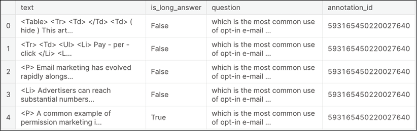
This is what the dataset looks like:
train.head()
tokenizer = text.Tokenizer(lower=False, num_words=80000)
for text in tqdm([train.text, test.text, train.question, test.question]):
    tokenizer.fit_on_texts(text.values)
train_target = train.is_long_answer.astype(int).values
train_text, train_questions, test_text, test_questions = compute_text_and_questions(train, test, tokenizer)
del train
We can now construct the model itself:
embedding_matrix = build_embedding_matrix(tokenizer, embedding_path)
model = build_model(embedding_matrix)
model.summary()
Model: "functional_1"
__________________________________________________________________________________________________
Layer (type)                    Output Shape         Param #     Connected to
==================================================================================================
input_1 (InputLayer)            [(None, None)]       0
__________________________________________________________________________________________________
input_2 (InputLayer)            [(None, None)]       0
__________________________________________________________________________________________________
embedding (Embedding)           (None, None, 300)    24000300    input_1[0][0]
                                                                 input_2[0][0]
__________________________________________________________________________________________________
spatial_dropout1d (SpatialDropo (None, None, 300)    0           embedding[0][0]
__________________________________________________________________________________________________
spatial_dropout1d_1 (SpatialDro (None, None, 300)    0           embedding[1][0]
__________________________________________________________________________________________________
bidirectional (Bidirectional)   (None, None, 200)    320800      spatial_dropout1d[0][0]
__________________________________________________________________________________________________
bidirectional_1 (Bidirectional) (None, None, 300)    541200      spatial_dropout1d_1[0][0]
__________________________________________________________________________________________________
global_max_pooling1d (GlobalMax (None, 200)          0           bidirectional[0][0]
__________________________________________________________________________________________________
global_max_pooling1d_1 (GlobalM (None, 300)          0           bidirectional_1[0][0]
__________________________________________________________________________________________________
concatenate (Concatenate)       (None, 500)          0           global_max_pooling1d[0][0]
                                                                 global_max_pooling1d_1[0][0]
__________________________________________________________________________________________________
dense (Dense)                   (None, 300)          150300      concatenate[0][0]
__________________________________________________________________________________________________
dropout (Dropout)               (None, 300)          0           dense[0][0]
__________________________________________________________________________________________________
dense_1 (Dense)                 (None, 300)          90300       dropout[0][0]
__________________________________________________________________________________________________
dropout_1 (Dropout)             (None, 300)          0           dense_1[0][0]
__________________________________________________________________________________________________
dense_2 (Dense)                 (None, 1)            301         dropout_1[0][0]
==================================================================================================
Total params: 25,103,201
Trainable params: 1,102,901
Non-trainable params: 24,000,300
__________________________________________________________________________________________________
The fitting is next, and that proceeds in the usual manner:
train_history = model.fit(
    [train_text, train_questions],
    train_target,
    epochs=2,
    validation_split=0.2,
    batch_size=1024
)
Now, we can build a test set to have a look at our generated answers:
directory = '/kaggle/input/tensorflow2-question-answering/'
test_path = directory + 'simplified-nq-test.jsonl'
test = build_test(test_path)
submission = pd.read_csv("../input/tensorflow2-question-answering/sample_submission.csv")
test_text, test_questions = compute_text_and_questions(test, tokenizer)
We generate the actual predictions:
test_target = model.predict([test_text, test_questions], batch_size=512)
test['target'] = test_target
result = (
    test.query('target > 0.3')
    .groupby('example_id')
    .max()
    .reset_index()
    .loc[:, ['example_id', 'PredictionString']]
)
result.head()
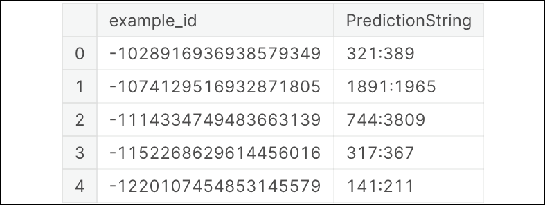
As you can see, LSTM allows us to handle fairly abstract tasks such as answering different types of questions. The bulk of the work in this recipe was around formatting the data into a suitable input format, and then postprocessing the results—the actual modeling occurs in a very similar fashion to that in the preceding chapters.
Summary
In this chapter, we have demonstrated the different capabilities of RNNs. They can handle diverse tasks with a sequential component (text generation and classification, time series prediction, and QA) within a unified framework. In the next chapter, we shall introduce transformers: an important architecture class that made it possible to reach new state-of-the-art results with NLP problems.