
11
Reinforcement Learning with TensorFlow and TF-Agents
TF-Agents is a library for reinforcement learning (RL) in TensorFlow (TF). It makes the design and implementation of various algorithms easier by providing a number of modular components corresponding to the core parts of an RL problem:
- An agent operates in an environment and learns by processing signals received every time it chooses an action. In TF-Agents, an environment is typically implemented in Python and wrapped in a TF wrapper to enable efficient parallelization.
- A policy maps an observation from the environment into a distribution over actions.
- A driver executes a policy in an environment for a specified number of steps (also called episodes).
- A replay buffer is used to store experience (agent trajectories in action space, along with associated rewards) of executing a policy in an environment; the buffer content is queried for a subset of trajectories during training.
The basic idea is to cast each of the problems we discuss as a RL problem, and then map the components into TF-Agents counterparts. In this chapter, we will show how TF-Agents can be used to solve some simple RL problems:
- The GridWorld problem
- The OpenAI Gym environment
- Multi-armed bandits for content personalization
The best way to start our demonstration of RL capabilities in TF-Agents is with a toy problem: GridWorld is a good choice due to its intuitive geometry and easy-to-interpret action but, despite this simplicity, it constitutes a proper objective, where we can investigate the optimal paths an agent takes to achieve the goal.
GridWorld
The code in this section is adapted from https://github.com/sachag678.
We begin by demonstrating the basic TF-Agents functionality in the GridWorld environment. RL problems are best studied in the context of either games (where we have a clearly defined set of rules and fully observable context), or toy problems such as GridWorld. Once the basic concepts are clearly defined in a simplified but non-straightforward environment, we can move to progressively more challenging situations.
The first step is to define a GridWorld environment: this is a 6x6 square board, where the agent starts at (0,0), the finish is at (5,5), and the goal of the agent is to find the path from the start to the finish. Possible actions are moves up/down/left/right. If the agent lands on the finish, it receives a reward of 100, and the game terminates after 100 steps if the end was not reached by the agent. An example of the GridWorld "map" is provided here:
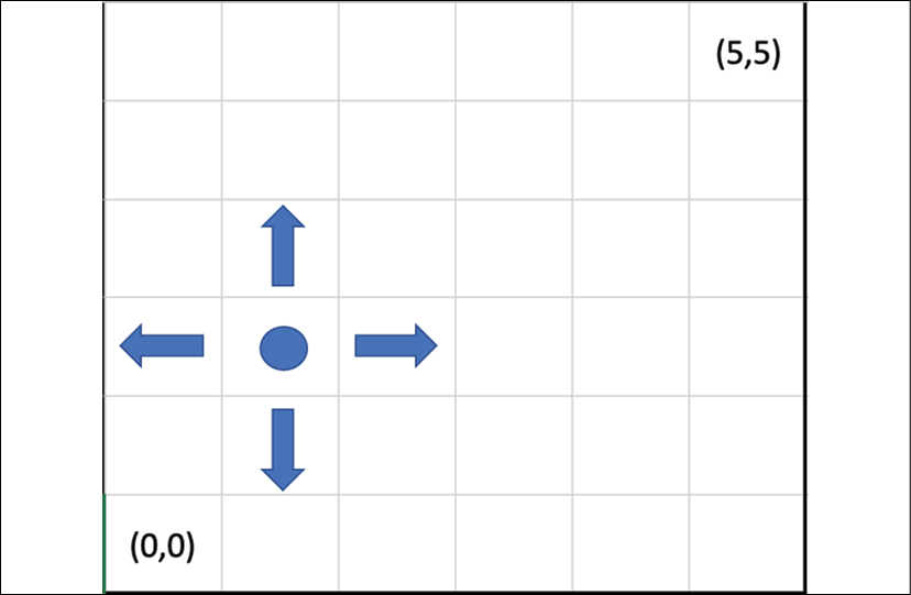
Figure 11.1: The GridWorld "map"
Now we understand what we're working with, let's build a model to find its way around the GridWorld from (0,0) to (5,5).
How do we go about it?
As usual, we begin by loading the necessary libraries:
import tensorflow as tf
import numpy as np
from tf_agents.environments import py_environment, tf_environment, tf_py_environment, utils, wrappers, suite_gym
from tf_agents.specs import array_spec
from tf_agents.trajectories import trajectory,time_step as ts
from tf_agents.agents.dqn import dqn_agent
from tf_agents.networks import q_network
from tf_agents.drivers import dynamic_step_driver
from tf_agents.metrics import tf_metrics, py_metrics
from tf_agents.policies import random_tf_policy
from tf_agents.replay_buffers import tf_uniform_replay_buffer
from tf_agents.utils import common
from tf_agents.drivers import py_driver, dynamic_episode_driver
from tf_agents.utils import common
import matplotlib.pyplot as plt
TF-Agents is a library under active development, so, despite our best efforts to keep the code up to date, certain imports might need to be modified by the time you are running this code.
A crucial step is defining the environment that our agent will be operating in. Inheriting from the PyEnvironment class, we specify the init method (action and observation definitions), conditions for resetting/terminating the state, and the mechanics for moving:
class GridWorldEnv(py_environment.PyEnvironment):
# the _init_ contains the specifications for action and observation
    def __init__(self):
        self._action_spec = array_spec.BoundedArraySpec(
            shape=(), dtype=np.int32, minimum=0, maximum=3, name='action')
        self._observation_spec = array_spec.BoundedArraySpec(
            shape=(4,), dtype=np.int32, minimum=[0,0,0,0],                            maximum=[5,5,5,5], name='observation')
        self._state=[0,0,5,5] #represent the (row, col, frow, fcol) of the player and the finish
        self._episode_ended = False
    def action_spec(self):
        return self._action_spec
    def observation_spec(self):
        return self._observation_spec
# once the same is over, we reset the state
    def _reset(self):
        self._state=[0,0,5,5]
        self._episode_ended = False
        return ts.restart(np.array(self._state, dtype=np.int32))
# the _step function handles the state transition by applying an action to the current state to obtain a new one
    def _step(self, action):
        if self._episode_ended:
            return self.reset()
        self.move(action)
        if self.game_over():
            self._episode_ended = True
        if self._episode_ended:
            if self.game_over():
                reward = 100
            else:
                reward = 0
            return ts.termination(np.array(self._state, dtype=np.int32),             reward)
        else:
            return ts.transition(
                np.array(self._state, dtype=np.int32), reward=0,                 discount=0.9)
    def move(self, action):
        row, col, frow, fcol = self._state[0],self._state[1],self._        state[2],self._state[3]
        if action == 0: #down
            if row - 1 >= 0:
                self._state[0] -= 1
        if action == 1: #up
            if row + 1 < 6:
                self._state[0] += 1
        if action == 2: #left
            if col - 1 >= 0:
                self._state[1] -= 1
        if action == 3: #right
            if col + 1 < 6:
                self._state[1] += 1
    def game_over(self):
        row, col, frow, fcol = self._state[0],self._state[1],self._        state[2],self._state[3]
        return row==frow and col==fcol
def compute_avg_return(environment, policy, num_episodes=10):
    total_return = 0.0
    for _ in range(num_episodes):
        time_step = environment.reset()
        episode_return = 0.0
        while not time_step.is_last():
            action_step = policy.action(time_step)
            time_step = environment.step(action_step.action)
            episode_return += time_step.reward
            total_return += episode_return
    avg_return = total_return / num_episodes
    return avg_return.numpy()[0]
def collect_step(environment, policy):
    time_step = environment.current_time_step()
    action_step = policy.action(time_step)
    next_time_step = environment.step(action_step.action)
    traj = trajectory.from_transition(time_step, action_step, next_time_step)
    # Add trajectory to the replay buffer
    replay_buffer.add_batch(traj)
We have the following preliminary setup:
# parameter settings
num_iterations = 10000
initial_collect_steps = 1000
collect_steps_per_iteration = 1
replay_buffer_capacity = 100000
fc_layer_params = (100,)
batch_size = 128 #
learning_rate = 1e-5
log_interval = 200
num_eval_episodes = 2
eval_interval = 1000
We begin by creating the environments and wrapping them to ensure that they terminate after 100 steps:
train_py_env = wrappers.TimeLimit(GridWorldEnv(), duration=100)
eval_py_env = wrappers.TimeLimit(GridWorldEnv(), duration=100)
train_env = tf_py_environment.TFPyEnvironment(train_py_env)
eval_env = tf_py_environment.TFPyEnvironment(eval_py_env)
For this recipe, we will be using a Deep Q-Network (DQN) agent. This means that we need to define the network and the associated optimizer first:
q_net = q_network.QNetwork(
        train_env.observation_spec(),
        train_env.action_spec(),
        fc_layer_params=fc_layer_params)
optimizer = tf.compat.v1.train.AdamOptimizer(learning_rate=learning_rate)
As indicated above, the TF-Agents library is under active development. The current version works with TF > 2.3, but it was originally written for TensorFlow 1.x. The code used in this adaptation was developed using a previous version, so for the sake of backward compatibility, we require a less-than-elegant workaround, such as the following:
train_step_counter = tf.compat.v2.Variable(0)
Define the agent:
tf_agent = dqn_agent.DqnAgent(
        train_env.time_step_spec(),
        train_env.action_spec(),
        q_network=q_net,
        optimizer=optimizer,
        td_errors_loss_fn = common.element_wise_squared_loss,
        train_step_counter=train_step_counter)
tf_agent.initialize()
eval_policy = tf_agent.policy
collect_policy = tf_agent.collect_policy
As a next step, we create the replay buffer and replay observer. The former is used for storing the (action, observation) pairs for training:
replay_buffer = tf_uniform_replay_buffer.TFUniformReplayBuffer(
        data_spec = tf_agent.collect_data_spec,
        batch_size = train_env.batch_size,
        max_length = replay_buffer_capacity)
print("Batch Size: {}".format(train_env.batch_size))
replay_observer = [replay_buffer.add_batch]
train_metrics = [
            tf_metrics.NumberOfEpisodes(),
            tf_metrics.EnvironmentSteps(),
            tf_metrics.AverageReturnMetric(),
            tf_metrics.AverageEpisodeLengthMetric(),
]
We then create a dataset from our buffer so that it can be iterated over:
dataset = replay_buffer.as_dataset(
            num_parallel_calls=3,
            sample_batch_size=batch_size,
    num_steps=2).prefetch(3)
The final bit of preparation involves creating a driver that will simulate the agent in the game and store the (state, action, reward) tuples in the replay buffer, along with storing a number of metrics:
driver = dynamic_step_driver.DynamicStepDriver(
            train_env,
            collect_policy,
            observers=replay_observer + train_metrics,
    num_steps=1)
iterator = iter(dataset)
print(compute_avg_return(eval_env, tf_agent.policy, num_eval_episodes))
tf_agent.train = common.function(tf_agent.train)
tf_agent.train_step_counter.assign(0)
final_time_step, policy_state = driver.run()
Having finished the preparatory groundwork, we can run the driver, draw experience from the dataset, and use it to train the agent. For monitoring/logging purposes, we print the loss and average return at specific intervals:
episode_len = []
step_len = []
for i in range(num_iterations):
    final_time_step, _ = driver.run(final_time_step, policy_state)
    experience, _ = next(iterator)
    train_loss = tf_agent.train(experience=experience)
    step = tf_agent.train_step_counter.numpy()
    if step % log_interval == 0:
        print('step = {0}: loss = {1}'.format(step, train_loss.loss))
        episode_len.append(train_metrics[3].result().numpy())
        step_len.append(step)
        print('Average episode length: {}'.format(train_metrics[3].                                                  result().numpy()))
    if step % eval_interval == 0:
        avg_return = compute_avg_return(eval_env, tf_agent.policy,                                        num_eval_episodes)
        print('step = {0}: Average Return = {1}'.format(step, avg_return))
Once the code executes successfully, you should observe output similar to the following:
step = 200: loss = 0.27092617750167847 Average episode length: 96.5999984741211 step = 400: loss = 0.08925052732229233 Average episode length: 96.5999984741211 step = 600: loss = 0.04888586699962616 Average episode length: 96.5999984741211 step = 800: loss = 0.04527277499437332 Average episode length: 96.5999984741211 step = 1000: loss = 0.04451741278171539 Average episode length: 97.5999984741211 step = 1000: Average Return = 0.0 step = 1200: loss = 0.02019939199090004 Average episode length: 97.5999984741211 step = 1400: loss = 0.02462056837975979 Average episode length: 97.5999984741211 step = 1600: loss = 0.013112186454236507 Average episode length: 97.5999984741211 step = 1800: loss = 0.004257255233824253 Average episode length: 97.5999984741211 step = 2000: loss = 78.85380554199219 Average episode length: 100.0 step = 2000:
Average Return = 0.0 step = 2200: loss = 0.010012316517531872 Average episode length: 100.0 step = 2400: loss = 0.009675763547420502 Average episode length: 100.0 step = 2600: loss = 0.00445540901273489 Average episode length: 100.0 step = 2800: loss = 0.0006154756410978734
While detailed, the output of the training routine is not that well suited for reading by a human. However, we can visualize the progress of our agent instead:
plt.plot(step_len, episode_len)
plt.xlabel('Episodes')
plt.ylabel('Average Episode Length (Steps)')
plt.show()
Which will deliver us the following graph:

Figure 11.2: Average episode length over number of episodes
The graph demonstrates the progress in our model: after the first 4,000 episodes, there is a massive drop in the average episode length, indicating that it takes our agent less and less time to reach the ultimate objective.
See also
Documentation for customized environments can be found at https://www.tensorflow.org/agents/tutorials/2_environments_tutorial.
RL is a huge field and even a basic introduction is beyond the scope of this book, but for those interested in learning more, the best recommendation is the classic Sutton and Barto book: http://incompleteideas.net/book/the-book.html
CartPole
In this section, we will make use of Open AI Gym, a set of environments containing non-trivial elementary problems that can be solved using RL approaches. We'll use the CartPole environment. The objective of the agent is to learn how to keep a pole balanced on a moving cart, with possible actions including a movement to the left or to the right:

Figure 11.3: The CartPole environment, with the black cart balancing a long pole
Now we understand our environment, let's build a model to balance a pole.
How do we go about it?
We begin by installing some prerequisites and importing the necessary libraries. The installation part is mostly required to ensure that we can generate visualizations of the trained agent's performance:
!sudo apt-get install -y xvfb ffmpeg
!pip install gym
!pip install 'imageio==2.4.0'
!pip install PILLOW
!pip install pyglet
!pip install pyvirtualdisplay
!pip install tf-agents
from __future__ import absolute_import, division, print_function
import base64
import imageio
import IPython
import matplotlib
import matplotlib.pyplot as plt
import numpy as np
import PIL.Image
import pyvirtualdisplay
import tensorflow as tf
from tf_agents.agents.dqn import dqn_agent
from tf_agents.drivers import dynamic_step_driver
from tf_agents.environments import suite_gym
from tf_agents.environments import tf_py_environment
from tf_agents.eval import metric_utils
from tf_agents.metrics import tf_metrics
from tf_agents.networks import q_network
from tf_agents.policies import random_tf_policy
from tf_agents.replay_buffers import tf_uniform_replay_buffer
from tf_agents.trajectories import trajectory
from tf_agents.utils import common
tf.compat.v1.enable_v2_behavior()
# Set up a virtual display for rendering OpenAI gym environments.
display = pyvirtualdisplay.Display(visible=0, size=(1400, 900)).start()
As before, there are some hyperparameters of our toy problem that we define:
num_iterations = 20000
initial_collect_steps = 100
collect_steps_per_iteration = 1
replay_buffer_max_length = 100000
# parameters of the neural network underlying at the core of an agent
batch_size = 64
learning_rate = 1e-3
log_interval = 200
num_eval_episodes = 10
eval_interval = 1000
Next, we proceed with function definitions for our problem. Start by computing the average return for a policy in our environment over a fixed period (measured by the number of episodes):
def compute_avg_return(environment, policy, num_episodes=10):
  total_return = 0.0
  for _ in range(num_episodes):
    time_step = environment.reset()
    episode_return = 0.0
    while not time_step.is_last():
      action_step = policy.action(time_step)
      time_step = environment.step(action_step.action)
      episode_return += time_step.reward
    total_return += episode_return
  avg_return = total_return / num_episodes
  return avg_return.numpy()[0]
Boilerplate code for collecting a single step and the associated data aggregation are as follows:
def collect_step(environment, policy, buffer):
  time_step = environment.current_time_step()
  action_step = policy.action(time_step)
  next_time_step = environment.step(action_step.action)
  traj = trajectory.from_transition(time_step, action_step, next_time_step)
  # Add trajectory to the replay buffer
  buffer.add_batch(traj)
def collect_data(env, policy, buffer, steps):
  for _ in range(steps):
    collect_step(env, policy, buffer)
If a picture is worth a thousand words, then surely a video must be even better. In order to visualize the performance of our agent, we need a function that renders the actual animation:
def embed_mp4(filename):
  """Embeds an mp4 file in the notebook."""
  video = open(filename,'rb').read()
  b64 = base64.b64encode(video)
  tag = '''
  <video width="640" height="480" controls>
    <source src="data:video/mp4;base64,{0}" type="video/mp4">
  Your browser does not support the video tag.
  </video>'''.format(b64.decode())
  return IPython.display.HTML(tag)
def create_policy_eval_video(policy, filename, num_episodes=5, fps=30):
  filename = filename + ".mp4"
  with imageio.get_writer(filename, fps=fps) as video:
    for _ in range(num_episodes):
      time_step = eval_env.reset()
      video.append_data(eval_py_env.render())
      while not time_step.is_last():
        action_step = policy.action(time_step)
        time_step = eval_env.step(action_step.action)
        video.append_data(eval_py_env.render())
  return embed_mp4(filename)
With the preliminaries out of the way, we can now proceed to actually setting up our environment:
env_name = 'CartPole-v0'
env = suite_gym.load(env_name)
env.reset()
In the CartPole environment, the following applies:
- An observation is an array of four floats:
- The position and velocity of the cart
- The angular position and velocity of the pole
- The reward is a scalar float value
- An action is a scalar integer with only two possible values:
- 0 — "move left"
- 1 — "move right"
As before, split the training and evaluation environments and apply the wrappers:
train_py_env = suite_gym.load(env_name)
eval_py_env = suite_gym.load(env_name)
train_env = tf_py_environment.TFPyEnvironment(train_py_env)
eval_env = tf_py_environment.TFPyEnvironment(eval_py_env)
Define the network forming the backbone of the learning algorithm in our agent: a neural network predicting the expected returns of all actions (commonly referred to as Q-values in RL literature) given an observation of the environment as input:
fc_layer_params = (100,)
q_net = q_network.QNetwork(
    train_env.observation_spec(),
    train_env.action_spec(),
    fc_layer_params=fc_layer_params)
optimizer = tf.compat.v1.train.AdamOptimizer(learning_rate=learning_rate)
train_step_counter = tf.Variable(0)
With this, we can instantiate a DQN agent:
agent = dqn_agent.DqnAgent(
    train_env.time_step_spec(),
    train_env.action_spec(),
    q_network=q_net,
    optimizer=optimizer,
    td_errors_loss_fn=common.element_wise_squared_loss,
    train_step_counter=train_step_counter)
agent.initialize()
Set up the policies – the main one used for evaluation and deployment, and the secondary one that is utilized for data collection:
eval_policy = agent.policy
collect_policy = agent.collect_policy
In order to have an admittedly not very sophisticated comparison, we will also create a random policy (as the name suggests, it acts randomly). This demonstrates an important point, however: a policy can be created independently of an agent:
random_policy = random_tf_policy.RandomTFPolicy(train_env.time_step_spec(), train_env.action_spec())
To get an action from a policy, we call the policy.action(time_step) method. The time_step contains the observation from the environment. This method returns a policy step, which is a named tuple with three components:
- Action: the action to be taken (move left or move right)
- State: used for stateful (RNN-based) policies
- Info: auxiliary data, such as the log probabilities of actions:
example_environment = tf_py_environment.TFPyEnvironment(
    suite_gym.load('CartPole-v0'))
time_step = example_environment.reset()
The replay buffer tracks the data collected from the environment, which is used for training:
replay_buffer = tf_uniform_replay_buffer.TFUniformReplayBuffer(
    data_spec=agent.collect_data_spec,
    batch_size=train_env.batch_size,
    max_length=replay_buffer_max_length)
For most agents, collect_data_spec is a named tuple called Trajectory, containing the specs for observations, actions, rewards, and other items.
We now make use of our random policy to explore the environment:
collect_data(train_env, random_policy, replay_buffer, initial_collect_steps)
The replay buffer can now be accessed by an agent by means of a pipeline. Since our DQN agent needs both the current and the next observation to calculate the loss, the pipeline samples two adjacent rows at a time (num_steps = 2):
dataset = replay_buffer.as_dataset(
    num_parallel_calls=3,
    sample_batch_size=batch_size,
    num_steps=2).prefetch(3)
iterator = iter(dataset)
During the training part, we switch between two steps, collecting data from the environment and using it to train the DQN:
agent.train = common.function(agent.train)
# Reset the train step
agent.train_step_counter.assign(0)
# Evaluate the agent's policy once before training.
avg_return = compute_avg_return(eval_env, agent.policy, num_eval_episodes)
returns = [avg_return]
for _ in range(num_iterations):
  # Collect a few steps using collect_policy and save to the replay buffer.
  collect_data(train_env, agent.collect_policy, replay_buffer, collect_steps_per_iteration)
  # Sample a batch of data from the buffer and update the agent's network.
  experience, unused_info = next(iterator)
  train_loss = agent.train(experience).loss
  step = agent.train_step_counter.numpy()
  if step % log_interval == 0:
    print('step = {0}: loss = {1}'.format(step, train_loss))
  if step % eval_interval == 0:
    avg_return = compute_avg_return(eval_env, agent.policy, num_eval_episodes)
    print('step = {0}: Average Return = {1}'.format(step, avg_return))
    returns.append(avg_return)
A (partial) output of the code block is given here. By way of a quick reminder, step is the iteration in the training process, loss is the value of the loss function in the deep network driving the logic behind our agent, and Average Return is the reward at the end of the current run:
step = 200: loss = 4.396056175231934
step = 400: loss = 7.12950325012207
step = 600: loss = 19.0213623046875
step = 800: loss = 45.954856872558594
step = 1000: loss = 35.900394439697266
step = 1000: Average Return = 21.399999618530273
step = 1200: loss = 60.97482681274414
step = 1400: loss = 8.678962707519531
step = 1600: loss = 13.465248107910156
step = 1800: loss = 42.33995056152344
step = 2000: loss = 42.936370849609375
step = 2000: Average Return = 21.799999237060547
Each iteration consists of 200 time steps and keeping the pole up gives a reward of 1, so our maximum reward per episode is 200:

Figure 11.4: Average return over number of iterations
As you can see from the preceding graph, the agent takes about 10 thousand iterations to discover a successful policy (with some hits and misses, as the U-shaped pattern of reward in that part demonstrates). After that, the reward stabilizes and the algorithm is able to successfully complete the task each time.
We can also observe the performance of our agents in a video. As regards the random policy, you can try the following:
create_policy_eval_video(random_policy, "random-agent")
And as regards the trained one, you can try the following:
create_policy_eval_video(agent.policy, "trained-agent")
See also
Open AI Gym environment documentation can be found at https://gym.openai.com/.
MAB
In probability theory, a multi-armed bandit (MAB) problem refers to a situation where a limited set of resources must be allocated between competing choices in such a manner that some form of long-term objective is maximized. The name originated from the analogy that was used to formulate the first version of the model. Imagine we have a gambler facing a row of slot machines who has to decide which ones to play, how many times, and in what order. In RL, we formulate it as an agent that wants to balance exploration (acquisition of new knowledge) and exploitation (optimizing decisions based on experience already acquired). The objective of this balancing is the maximization of a total reward over a period of time.
An MAB is a simplified RL problem: an action taken by the agent does not influence the subsequent state of the environment. This means that there is no need to model state transitions, credit rewards to past actions, or plan ahead to get to rewarding states. The goal of an MAB agent is to determine a policy that maximizes the cumulative reward over time.
The main challenge is an efficient approach to the exploration-exploitation dilemma: if we always try to exploit the action with the highest expected rewards, there is a risk we miss out on better actions that could have been uncovered with more exploration.
The setup used in this example is adapted from the Vowpal Wabbit tutorial at https://vowpalwabbit.org/tutorials/cb_simulation.html.
In this section, we will simulate the problem of personalizing online content: Tom and Anna go to a website at different times of the day and are shown an article. Tom likes politics in the morning and music in the afternoon, while Anna prefers sport or politics in the morning and politics in the afternoon. Casting the problem in MAB terms, this means the following:
- The context is a pair {user, time of day}
- Possible actions are news topics {politics, sport, music, food}
- The reward is 1 if a user is shown content they find interesting at this time, and 0 otherwise
The objective is to maximize the reward measured through the clickthrough rate (CTR) of the users.
How do we go about it?
As usual, we begin by loading the necessary packages:
!pip install tf-agents
import abc
import numpy as np
import tensorflow as tf
from tf_agents.agents import tf_agent
from tf_agents.drivers import driver
from tf_agents.environments import py_environment
from tf_agents.environments import tf_environment
from tf_agents.environments import tf_py_environment
from tf_agents.policies import tf_policy
from tf_agents.specs import array_spec
from tf_agents.specs import tensor_spec
from tf_agents.trajectories import time_step as ts
from tf_agents.trajectories import trajectory
from tf_agents.trajectories import policy_step
tf.compat.v1.reset_default_graph()
tf.compat.v1.enable_resource_variables()
tf.compat.v1.enable_v2_behavior()
nest = tf.compat.v2.nest
from tf_agents.bandits.agents import lin_ucb_agent
from tf_agents.bandits.environments import stationary_stochastic_py_environment as sspe
from tf_agents.bandits.metrics import tf_metrics
from tf_agents.drivers import dynamic_step_driver
from tf_agents.replay_buffers import tf_uniform_replay_buffer
import matplotlib.pyplot as plt
We then define some hyperparameters that will be used later:
batch_size = 2
num_iterations = 100
steps_per_loop = 1
The first function we need is a context sampler to generate observations coming from the environment. Since we have two users and two parts of the day, it comes down to generating two-element binary vectors:
def context_sampling_fn(batch_size):
  def _context_sampling_fn():
    return np.random.randint(0, 2, [batch_size, 2]).astype(np.float32)
  return _context_sampling_fn
Next, we define a generic function for calculating the reward per arm:
class CalculateReward(object):

    """A class that acts as linear reward function when called."""
    def __init__(self, theta, sigma):
        self.theta = theta
        self.sigma = sigma
    def __call__(self, x):
        mu = np.dot(x, self.theta)
        #return np.random.normal(mu, self.sigma)
        return (mu > 0) + 0
We can use the function to define the rewards per arm. They reflect the set of preferences described at the beginning of this recipe:
arm0_param = [2, -1]
arm1_param = [1, -1]
arm2_param = [-1, 1]
arm3_param = [ 0, 0]
arm0_reward_fn = CalculateReward(arm0_param, 1)
arm1_reward_fn = CalculateReward(arm1_param, 1)
arm2_reward_fn = CalculateReward(arm2_param, 1)
arm3_reward_fn = CalculateReward(arm3_param, 1)
The final part of our function's setup involves a calculation of the optimal rewards for a given context:
def compute_optimal_reward(observation):
    expected_reward_for_arms = [
      tf.linalg.matvec(observation, tf.cast(arm0_param, dtype=tf.float32)),
      tf.linalg.matvec(observation, tf.cast(arm1_param, dtype=tf.float32)),
      tf.linalg.matvec(observation, tf.cast(arm2_param, dtype=tf.float32)),
      tf.linalg.matvec(observation, tf.cast(arm3_param, dtype=tf.float32))
    ]
    optimal_action_reward = tf.reduce_max(expected_reward_for_arms, axis=0)

    return optimal_action_reward
For the sake of this example, we assume that the environment is stationary; in other words, the preferences do not change over time (which does not need to be the case in a practical scenario, depending on your time horizon of interest):
environment = tf_py_environment.TFPyEnvironment(
    sspe.StationaryStochasticPyEnvironment(
        context_sampling_fn(batch_size),
        [arm0_reward_fn, arm1_reward_fn, arm2_reward_fn, arm3_reward_fn],
        batch_size=batch_size))
We are now ready to instantiate an agent implementing a bandit algorithm. We use a predefined LinUCB class; as usual, we define the observation (two elements representing the user and the time of day), time step, and action specification (one of four possible types of content):
observation_spec = tensor_spec.TensorSpec([2], tf.float32)
time_step_spec = ts.time_step_spec(observation_spec)
action_spec = tensor_spec.BoundedTensorSpec(
    dtype=tf.int32, shape=(), minimum=0, maximum=2)
agent = lin_ucb_agent.LinearUCBAgent(time_step_spec=time_step_spec,
                                     action_spec=action_spec)
A crucial component of the MAB setup is regret, which is defined as the difference between an actual reward collected by the agent and the expected reward of an oracle policy:
regret_metric = tf_metrics.RegretMetric(compute_optimal_reward)
We can now commence the training of our agent. We run the trainer loop for num_iterations and execute steps_per_loop in each step. Finding the appropriate values for those parameters is usually about striking a balance between the recent nature of updates and training efficiency:
replay_buffer = tf_uniform_replay_buffer.TFUniformReplayBuffer(
    data_spec=agent.policy.trajectory_spec,
    batch_size=batch_size,
    max_length=steps_per_loop)
observers = [replay_buffer.add_batch, regret_metric]
driver = dynamic_step_driver.DynamicStepDriver(
    env=environment,
    policy=agent.collect_policy,
    num_steps=steps_per_loop * batch_size,
    observers=observers)
regret_values = []
for _ in range(num_iterations):
    driver.run()
    loss_info = agent.train(replay_buffer.gather_all())
    replay_buffer.clear()
    regret_values.append(regret_metric.result())
We can visualize the results of our experiment by plotting the regret (negative reward) over subsequent iterations of the algorithm:
plt.plot(regret_values)
plt.ylabel('Average Regret')
plt.xlabel('Number of Iterations')
Which will plot the following graph for us:

Figure 11.5: Performance of a trained UCB agent over time
As the preceding graph demonstrates, after an initial period of learning (indicating a spike in regret around iteration 30), the agent keeps getting better at serving the desired content. There is a lot of variation going on, which shows that even in a simplified setting – two users – efficient personalization remains a challenge. Possible avenues of improvement could involve longer training or adapting a DQN agent so that more sophisticated logic can be employed for prediction.
See also
An extensive collection of bandits and related environments can be found in the TF-Agents documentation repository: https://github.com/tensorflow/agents/tree/master/tf_agents/bandits/agents/examples/v2.
Readers interested in contextual multi-armed bandits are encouraged to follow the relevant chapters from the book by Sutton and Barto: https://web.stanford.edu/class/psych209/Readings/SuttonBartoIPRLBook2ndEd.pdf.