
Online recommendation systems used by Netflix and Amazon
Trendy self-driving cars from Tesla and Alphabet
Fraud detection solutions for banks and e-commerce merchants
Machine learning algorithms for medical diagnosis and prediction
Sentiment analyzer on social media to provide digital consumer insights
This chapter explores the issues and challenges of machine learning development and deployment. It covers some of the key requirements and design considerations behind ML deployment solutions. Finally, it dives into specific solution components, best practices, and tooling.
ML Development Challenges
Like any software solution, model-driven applications are measured using common software quality characteristics, such as functionality, reliability, maintainability, scalability, and performance. ML applications must address all the quality issues of traditional software plus an additional set of ML-specific requirements. Therefore, ML application development is harder than traditional software development.
Classical Software Engineering vs. Machine Learning
In classical software engineering settings, the desired product behavior can be sufficiently expressed in software logic alone. Once the coded logic is thoroughly tested in user scenarios with mock data, the code is expected to continue to work with the real data in the production environment.
On the contrary, an ML application learns to perform a task without being specifically programmed. Its quality depends on the input data and tuning parameters. When a model is trained, a mapping function is established between the input (i.e., independent variables) to the output (i.e., target variables). This mapping learned from historical data may not always be valid in the future on new data if the relationships between input and output data have changed. This change can have detrimental effects on the dependent applications or services because the model predictions become less accurate as time passes. An ML application must be fed new data to keep working.
Model Drift
The concept of model drift means that, over time, changing external data results in poor and degrading predictive performance in predictive models. Depending on the cause of the drift, model drift can be categorized into two types: concept drift and data drift.
Concept drift refers to the change in the statistical properties of the target variable change over time. Email spam filtering application exhibits frequent concept drift due to the evolving nature of spam and legitimate emails.
While concept drift is about the target variable, data drift occurs when properties of independent variables change. For instance, a data set contains information on default payments, demographic factors, credit data, history of payment, and bill statements of credit card clients. A machine learning model can be trained to predict the likelihood of credit card default for customers in the bank. In this case, it is not the definition of the target variable (default payment) that changes but the values of independent variables (demographic factors, credit data, history of payment, and bill statements) that define the target.
In machine learning, features or attributes are independent variables input for the machine learning algorithm to analyze. A target (the output) is the dependent variable about which you want to gain a deeper understanding. In the context of a supervised classification model, the term class label refers to a unique value of the target.
ML Deployment Challenges
As data scientists and software engineers continue to accumulate experience with live ML systems, you can gain a greater understanding of the unique challenges, how they happen, their implications, and how to overcome the challenges.
ML life cycle and key artifacts
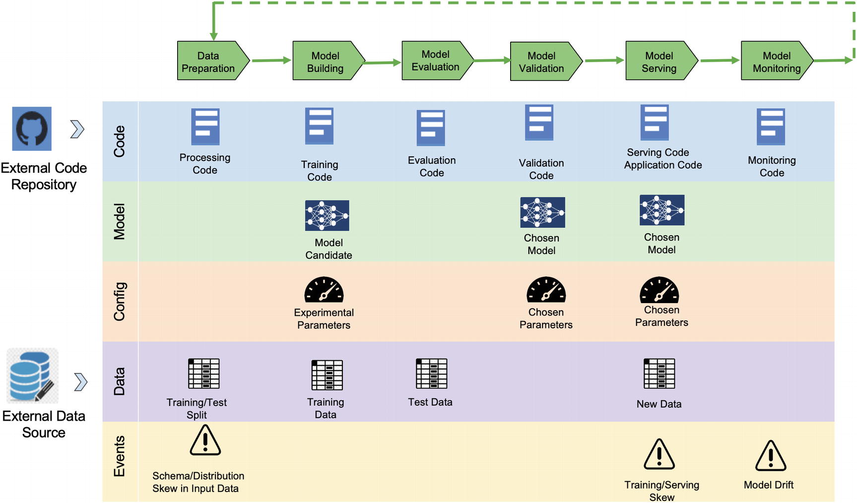
For models that deal with live data, model training does not end at model development. Once operational, models need to be monitored, and frequent model retraining may be required to keep up with changing circumstances. A retraining pipeline with model monitoring needs to be added to feed the model serving module, resulting in the life cycle pattern in Figure 8-1.
ML Life Cycle
The ultimate goal of deploying and maintaining live ML-driven applications is to maintain optimal model performance metrics (such as loss, accuracy). This requires constant experimentation/validation to improve metrics due to changes in live data. To make this task more challenging, the improvement needs to be automated.
As described in Figure 8-1, each iteration of the ML life cycle is associated with a specific version of the source code (including versioned dependent libraries) pushed from an external repository. Also, the iteration accesses input data from an external data source which is also versioned.
Data preparation: Data processing code first validates the raw data and generates events if schema or distribution skew detected. Otherwise, the data is pre-processed and split into a training set and a test set.
Model building: A candidate model is created with experimental parameters. This model is trained using the training set.
Model evaluation: The candidate model is evaluated, and performance metrics are produced.
Model validation: The candidate model is validated/compared with the current live version. The validation code chooses a version that better meets the performance requirement.
Model serving: The model serving code promotes the chosen model to production to serve predictions using new data.
Model monitoring: In this phase, schema or distribution skews (in features and predictions) are detected by comparing consecutive spans of historical data sets. For instance, if data ingestion happens monthly, you compare between consecutive months of training data. Model drift events are logged if notable drift is detected, which triggers model retraining by starting a new iteration of the life cycle.
Scaling Challenges
Data scientists and data engineers focus on several key areas when it comes to scaling machine learning solutions.
Model Training
During training, a series of mathematical computations are applied to massive amounts of data repeatedly. Training such a model to reach a decent accuracy can take a long time (days or weeks). This problem is multiplied by the number of models to be trained.
Model Inference
Model inference service has to handle many inputs or users and meet latency and throughput requirements. For accelerating deep learning inference in computer vision, optimization is required in both hardware and application levels.
Input Data Processing
Throughout a typical ML life cycle, a massive amount of data is fed to the system. The memory representation and the way algorithms access data can have a significant impact on scalability. Furthermore, to keep up with the data consumption rate of multiple accelerated hardware devices, the data processing speed and throughput must be scaled up.
Key Requirements
Automation of the entire ML life cycle (with the possibility of human intervention/approval when required).
Tracking and managing ML models and artifacts such as data, code, model packages, configuration, dependencies, and performance metrics are critical for drift detection, model reproducibility, auditability, debugging, and explainability.
Model performance (such as accuracy) is the key quality indication of any ML model.
ML operational requirements include ML API endpoints response time, Memory/CPU usage when performing prediction, and disk utilization (if applicable).
Design Considerations and Solutions
To overcome challenges and meet the set of requirements, let’s discuss common design considerations and recent advances in solutions and tooling.
Automating Data Science Steps
Typically, productizing any ML model requires automating the life-cycle processing, which translates to the following specific data science steps.
Data ingestion/pre-processing: Collect and process raw data from incoming data sources.
Data validation: Verify the input data schema and statistical properties are as expected by the model.
Data preparation: Clean, normalize, and split the data into training/test sets.
Feature engineering: Transform raw data to construct additional features that better represent the underlying problem to the model.
Feature selection: Remove irrelevant features and select those features which contribute most to the target variable. The output of this step is the feature splits in the format expected by the training algorithm.
Model training: Apply various ML algorithms to the prepared feature set to train ML models. This includes hyperparameter tuning to get the best performing ML model. The output of this step is a trained model.
Model evaluation: Assess the quality of the trained model using a set of metrics.
Model validation: Determine whether the model is adequate for deployment based on model evaluation and monitoring metrics.
Model serving: The ML inference program uses a trained model to generate predictions.
Model monitoring: Monitor to detect training/serving skew and model drift. If the drift is significant, the model must be retrained and refreshed with more recent data.
These manual data science steps must be reflected in an automated pipeline before the pipeline can be deployed in any production environment. MLOps is an important and relatively new concept in the context of ML automation. Let’s introduce MLOps and then dive into key solutions that are enabled within the MLOps framework.
Automated ML Pipeline: MLOps
MLOps (a compound of machine learning and operations) is a set of practices that combines the practices between data scientists and operations professionals to automate and manage the production ML (or deep learning) life cycle. MLOps is a CI/CD framework for large-scale machine learning productization.
Continuous integration (CI) is a software development best practice for merging all developers' working copies to a shared repository frequently, preferably several times a day. Each merge can then be verified by an automated build and automated acceptance tests.Continuous delivery (CD) is the practice of keeping your codebase deployable at any point. Beyond making sure your application passes automated tests, it must have all the configuration, dependencies, and packaging necessary to push it into production.
DevOps is a set of practices that automate and integrate the processes between classical software development and operations teams. DevOps combines cultural philosophies, practices, and tools to increase an organization’s ability to deliver high-velocity applications and services.
Git: A source code repository
Jenkins: An automation facility
Kubeflow and Airflow: Orchestrators
Travis CI: A continuous integration service
Argo CD: A continuous delivery tool
Kubernetes: A container-orchestration system for automating application deployment
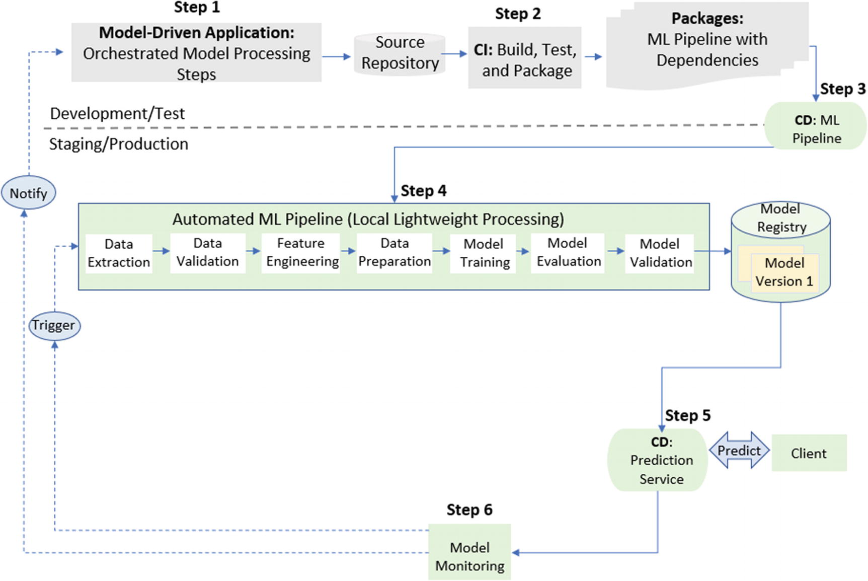
Figure 8-2 shows a model-driven application code contains an ML pipeline (step 1).
Once the code is committed and merged in the code repository (Git), DevOps’ continuous integration tool automatically starts the integration and testing (step 2).
ML pipeline automation
Special hardware: Special segmentation and orchestration of data and algorithm required to take advantage of accelerated hardware (such as Graphics Processing Units (GPUs) and Tensor Processing Units (TPU)) and meet scalability requirements.
- Complex computational graphs: Orchestration can involve complex runtime computational graphs. ML applications can have multiple pipelines executing in parallel.
A/B testing
Ensembles
Multi-armed bandits
Reproducibility: Due to the experimental nature of model training, it is important to maintain repeatability for pipelines and components. The ML pipelines can be reused, adjusted, resumed using the information in the model registry. For instance, a pipeline can skip some steps or resume an intermediate step (step 4).
Continuous model delivery: Once the model registry decides to raise a model from staging to production, the model is automatically made ready to be consumed by the Prediction Service and the downstream application/client (step 5). This step enables the “continuous delivery” of new model versions within an ML pipeline, which overrides the regular DevOps process (step 3). Additional ML-specific interdependencies such as model registry, model refresh management, model validation, data validation, or drift detection.
Regulatory compliance: Additional explainability and interpretability modules must articulate model intricacies to address various compliance regulators.
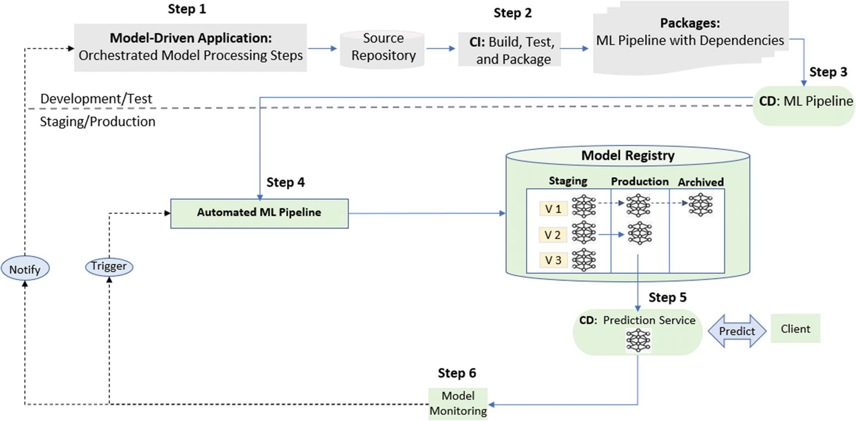
Model Registry for Tracking
The model registry component is a centralized data store that supports the management of the full life cycle of ML models. It provides model versioning, production/stage/archived transitions, tracking for data dependency, code dependency, environment, and configuration for every active pipeline instance.
Model registry example
The selected version of the trained model
The version of input data (the version to identify the raw input data)
The version of code (versions of all source code—model training, application, pipeline processing, etc.—as tracked in the external source code repository)
Dependencies (linkage to dependent libraries, database connections, etc.)
Environment configuration (parameters to control ML pipeline components, such as data processing, feature selection, the threshold value used by data validation or model monitoring)
Hyperparameters (a parameter whose value controls the ML learning process; e.g., learning rate, batch size, size of a neural network, number of epochs, number of layers, number of filters, and optimizer name)
Trained model packages(the resulting package from model training. Typical formats are pickle, ONNX, and PMML)
Model scoring results (the predictions made by the model)
Features for training and testing
Feature importance (the score assigned to input features based on how useful they are at predicting a target variable)
- Model performance metrics
Training time
Accuracy
Loss
Confusion matrix (see Figure 8-4)
Accuracy: (TP+TN)/(TP+FP+TN+FN)
Precision: TP/(TP+FP)
Recall: TP/(TP+FN)
TP is the number of cases that were predicted to be true, and the actual result is True.
TN is the number of cases that were predicted to be True, but the actual result is False.
FP is the number of cases that were predicted to be False, but the actual result is True.
FN is the number of cases that were predicted to be False, and the actual result is False.
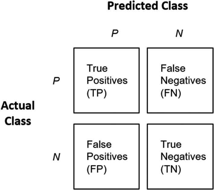
Model evaluation: confusion matrix from binary classification
By storing the information in the model registry, it is possible to reproduce any model training. You can also monitor a series of training instances to detect any regression and choose to redeploy or even roll back all or parts of the pipeline in production.
Data Validation
As the rapid application of ML models to key areas of our daily life, it is important to explain the reasoning behind the model predictions. However, there is no easy way to effectively examine the internal structure of a trained model for correctness to justify unintended model behavior.
By comparison, validating the data is much more straightforward. The input data is the starting point of the ML pipeline, so data validation should be the first line of defense to flag problems before the entire pipeline is activated with poor data.
The current data set conforms to the same schema as the previous data set.
The feature values of the current data set are similar to those of the previous data set.
The feature value distributions of the current data set are similar to those of the previous data set.
Other model-specific patterns are unchanged. For example, in a Natural Language Processing (NLP) scenario, a sudden change in the number of words and the list of words not seen in the previous data set.
The serving data set and the training data set conform to the same schema.
The feature values that the model trains on are similar to the feature values that it sees at the serving time.
The feature value distributions for the training data set are similar to those of the serving data set.
Other model-specific patterns are unchanged. For example, in an NLP scenario, a sudden change in the number of words and the list of words in the serving data not seen in the training data.
Pipeline Abstraction
Data transformation
Data normalization
Model invocation
Algorithm selection
Term frequency–Inverse document frequency (TF-IDF) weighting
Automatic Machine Learning (AutoML)
While the pipeline abstraction aims to deduplicate and optimize the code structure, AutoML seeks to automate the many cumbersome and repetitive steps or groups of steps in the pipeline during runtime.
With AutoML, people with limited machine learning expertise can take advantage of the state-of-the-art modules. AutoML also frees model developers from the burden of repetitive and time-consuming tasks.
Data pre-processing
Data partitioning
Feature extraction
Feature selection
Algorithm selection
Training
Tuning
Ensembling
Deployment
Monitoring
Model Monitoring
How do you know your models in production are behaving as you expect them to? What are the impacts on your model and the downstream application when your training data becomes stale? How does your ML pipeline handle corrupted live data or training/serving skew?
To begin addressing these complex issues, metrics and artifacts representing the raw measurements of performance or behavior are observed and collected throughout your systems. For each pipeline execution instance, model packages, metrics, and other artifacts are persisted in a model registry. Model registry is covered in more detail later in this chapter.
Using the information in the model registry, the model monitoring component can reproduce the pipeline execution, conduct a detailed comparison of the current and historical instances to detect data deviation, model drift, dependency changes, and conduct production A/B testing.
Model Monitoring Implementation
Schema of incoming raw data
Distribution of incoming raw data
Model prediction distribution for regression algorithms or prediction frequencies for classification algorithms
Model feature distribution for numerical features or input frequencies for categorical features
Missing value checks
Model performance metrics (loss, accuracy, etc.)
Median and mean values over a given timeframe
Min/Max values
Standard deviation over a given timeframe
If the monitoring component detects a significant drift, it triggers the restart of the ML pipeline with more recent input data. The resulting model instances are placed in staging. The model validation module then decides to refresh the model in production.
In dependency change, the monitoring module notifies the data scientist to request human intervention/approval.
Scaling Solutions
ML applications require specific hardware configurations and scalability considerations. For example, training neural networks can require powerful GPUs. Training common machine learning models can require clusters of CPUs. To take advantage of the accelerated hardware, the ML model and input data need to be partitioned, sized, configured, and mapped a cluster of computational nodes (running ML frameworks such as Spark, scikit-learn, and PyTorch).
ML Accelerators for Large Scale Model Training and Inference
GPUs (graphics processing units) contain hundreds of embedded ALUs that handle parallelized computations.
Application-specific integrated circuits (ASICs) such as Google’s TPUs are matrix processors designed for deep learning.
Intel’s Habana Goya and Gaudi chips: Gaudi for training and Goya for inference.
Distributed Machine Learning for Model Training
Distributed machine learning refers to multi-node/multi-processor machine learning algorithms and systems designed to improve training performance, accuracy, and scale to larger input data sizes. Data parallelism and model parallelism are different ways of distributing the workload across nodes. Data parallelism is when you run the algorithm in every node but feed it with different parts of the partitioned data; model parallelism is when you use the same data for every node but split the model among nodes.
Apache Hadoop (HDFS)
Apache Spark (MLlib)
Apache Mahout
TensorFlow and PyTorch: Frameworks with APIs for distributed computation by model/data parallelism
Model Inference Options
REST endpoints
Traditional batch inference operations
Distributed stream processing systems, such as Spark Streaming or Apache Flink
Parallelizing ML inferences across all available nodes/accelerated devices can reduce the overall inference time. Other inference optimization methods batch-size adjustment and model pruning.
graphics processing units (GPU)
field-programmable gate arrays (FPGA)
vision processing units (VPU)
Input Data Pipeline

Performance bottleneck: input data pipeline
Extract is the process of reading data from multiple and often different types of sources. This stage is I/O intensive.
Transform is the process of applying rules to convert/combine the extracted data into the desired format. This stage is compute-intensive and typically handled by CPUs.
Load is the process of writing the data into the target datastore and ready to be fed to the training algorithm. This stage is also I/O intensive.

Sequential input data pipeline
Parallelize file/database reading during the extract phase
Parallelize transformation operations (shuffle, map, etc.) across multiple CPU cores
Prefetch pipelines and operations for training
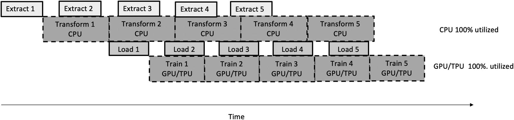
Parallel (optimized) input data pipeline
ML Tooling Ecosystem
In the beginning of the chapter, we introduced the concept of machine learning pipeline and pipeline automation. As described in Figure 8-2, the machine learning pipeline consists of two distinct phases: Model Development (steps 1, 2, and 3) and Model Deployment (steps 4, 5, and 6).
Figure 8-8 provides an overview of the tooling landscape in the machine learning space, where we group tools according to phases: The Model Development / Training (bottom left) and Model Serving (bottom right) are specific frameworks/libraries/modules supporting Model Development and Model Deployment phases, respectively.
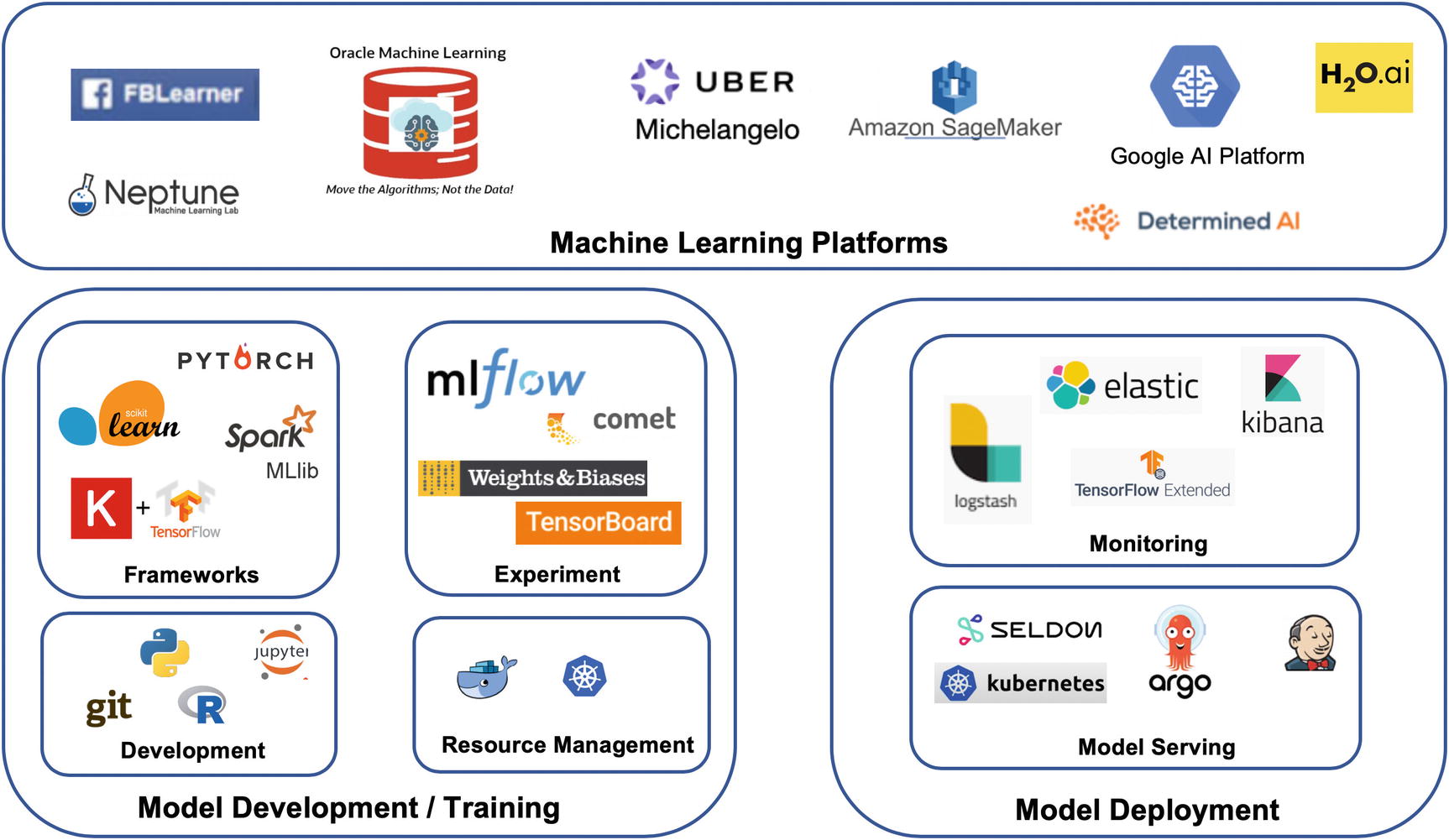
Machine learning tools
ML Platforms
Amazon SageMaker
Facebook FBLearner
Oracle Machine Learning
Uber Michelangelo
Google AI Platform
Neptune
Next, let’s go over ML Development tools. Tools in the Model Development/Training group can be divided into categories such as ML Frameworks, Development Environments, Experiment Tracking, and Resource Management.
ML Development Tools
TensorFlow
Keras
scikit-learn
PyTorch
Spark MLlib
In the Development Environments category, Jupyter notebook, Python, R are popular among data scientists. Git is a distributed version control system.
For experiment management, we have mlflow for tracking. Tensorboard is very useful for tracking and visualizing metrics as well as model graphs. More information about tensorboard can be found here: https://www.tensorflow.org/tensorboard/get_started.
For resource management, Docker and Kubernetes can be used to define and customize a set of resource usage conditions and policies during data processing and model training.
Since 2016, as large amounts of data and off-the-shelf models become more accessible, the demand for tools to help productize/deploy machine learning increases. As shown in Figure 8-8, the Deployment tools can be divided into Model Monitoring and Model Serving categories.
ML Deployment Tools
Seldom
Argo
Kubernetes
Jenkins
In addition, monitoring tools such as the following are commonly deployed to handle/visualize model drift and data anomaly detection.
TensorFlow Data Validation
Logstash
Elasticsearch
Kibana
Summary
This chapter analyzed the challenges of deploying and machine learning model-driven applications. We went through key requirements, important concepts, high-level architecture, and design considerations. We discussed machine learning deployment infrastructure and solutions. The chapter ended with a summary of tooling supporting the ML pipeline life cycle.