
Oracle Advanced Analytics consists of Oracle Data Mining and Oracle R Enterprise. On December 5, 2019, Oracle announced Advanced Analytics functionality as a cost-free option. Now, Oracle Data Mining has been rebranded to Oracle Machine Learning for SQL (OML4SQL), Oracle R Enterprise (ORE) to Oracle Machine Learning for R (OML4R) and Oracle R Advanced Analytics for Hadoop (OML4Spark).
New members of the OML family were also introduced. Oracle Machine Learning for Python (OML4Py), OML Microservices for Oracle applications, and Oracle Machine Learning Notebooks, Apache Zeppelin–inspired notebooks in Oracle Autonomous Database. This chapter discusses OML4SQL.
OML4SQL is a set of PL/SQL packages for machine learning implemented in Oracle Database. It is very convenient for Oracle professionals because all the knowledge they have gathered during the years working on Oracle technologies is still valid and very useful when learning new skills on machine learning. In OML4SQL, data is stored in a database or external tables, and the machine learning algorithms are inside the database. Instead of moving the data to be processed for machine learning, it stays where it is, and the processing is done there.
Moving data is often time-consuming and complicated. And what would be a better place to process data than a database. Since the data stays in the database, the security, backups, and so forth are managed by the database management system. The security risks related to moving data have been eliminated.
Having machine learning elements such as the model as a first-class citizen of the database makes handling them easy and similar to the handling process of any other database object. For instance, models can be trained in parallel. They can be exported from the test database and imported to the production database, and privileges can be defined easily and fine-grained.
Being able to do machine learning in a database brings a lot of advantages and fastens the process. However, the disadvantages are that the selection of algorithms depends on the database version, and adding new algorithms might be considered complicated. Though a simple solution usually yields the best result and existing algorithms are enough: good quality data, quick experiments, feature engineering, and model tuning rather than applying fundamentally different algorithms brings the largest improvements.
In Oracle Machine Learning, a feature (e.g., name or age) is called an attribute. A method (e.g., classification or clustering) is called a machine learning function. OML4SQL supports supervised and unsupervised machine learning. It supports neural networks and text processing, but it does not support convolutional neural networks and visual recognition problems.
PL/SQL Packages for OML4SQL
DBMS_PREDICTIVE_ANALYTICS routines for performing semi-automized machine learning using predictive analytics
DBMS_DATA_MINING_TRANSFORMING routines for transforming the data for OML4SQL algorithms
DBMS_DATA_MINING routines for creating and managing the machine learning models and evaluating them
All of them have several subprograms, which are discussed later in this chapter.
Privileges
The three OML4SQL packages are owned by the SYS user. They are part of the database installation. The installation also includes granting the execution privilege on the packages to the public. When the routines in the package are run, it’s done with those privileges the current user has (invoker’s privileges). To use OML4SQL in an Oracle Autonomous Database, create the user using the Manage Oracle ML Users functionality in Administration functionality under Service Console. Oracle automatically adds the necessary privileges.
CREATE SESSION
CREATE TABLE
CREATE VIEW
ALTER ANY MINING MODEL
DROP ANY MINING MODEL
SELECT ANY MINING MODEL
COMMENT ANY MINING MODEL
AUDIT ANY MINING MODEL
If the user needs to do processing with text type data, EXECUTE ON ctxsys.ctx_ddl privilege is needed because OML4SQL uses Oracle Text functionalities when processing text.
It is also possible to grant individual object privileges on existing machine learning models. Designing the privileges is an important step of the process, and it is possible the privileges in the test environment will be different from those in the production environment.
Data Dictionary Views
_MINING_MODELS
_MINING_MODEL_ATTRIBUTES
_MINING_MODEL_PARTITIONS
_MINING_MODEL_SETTINGS
_MINING_MODEL_VIEWS
_MINING_MODEL_XFORMS
Let’s use the USER_ view set as an example to investigate these views. USER_MINING_MODELS view has all the information about models created by the user who has logged in to the database. It includes the name of the model, what function was used, what algorithm was used, the algorithm type, creation date, duration of building the model, size of the model, is the model partitioned or not, and some optional comments about the model.
The view USER_MINING_MODEL_ATTRIBUTES describes all the attributes used when building the model. It includes information about the name of the model, name of the attribute, type of the attribute (categorical/numeric), datatype, length, precision, scale, usage type, information on whether this attribute is the target, and optional specifications for the attribute.
The view USER_MINING_MODEL_SETTINGS includes all the settings defined for models. The view includes the name of the model, the setting name and value, and a setting type indicating whether it is defined by the user with a settings table (INPUT) or is the default value (DEFAULT). The settings tables are discussed later in this chapter.
USER_MINING_MODEL_VIEWS includes information about all the views the machine learning process has created. These views are called model detail views. These views have been in a database since Oracle Database 12.2. They are for inspecting a model’s details. USER_MINING_MODEL_VIEWS includes the name of the model, the name of the view, and the view type. The name of the view always starts with DM. The view types include Scoring Cost Matrix, Model Build Alerts, Classification Targets, Computed Settings, and Decision Tree Hierarchy. The views created depend on the algorithm.
USER_MINING_MODEL_XFORMS view describes the user-specified transformations embedded models. This is discussed later in this chapter.
USER_MINING_MODEL_PARTITIONS includes data about a partitioned model, which is covered later in this chapter.
Predictive Analytics
EXPLAIN
PREDICT
PROFILE
EXPLAIN ranks attributes in order of their influence in explaining the target column; in other words, it calculates the attribute importance. PREDICT predicts the value of a target column using the values in the input data. PROFILE generates rules that describe the cases from the input data. All mining activities are handled internally by these procedures, but at least some of the rows in the data set must have data on the target column.
Ten of the columns have some importance in predicting the target attribute. Eight of them have no importance at all. If you carefully look at the results, you see that the most important columns (taste, palate, aroma, appearance) are null in a new data set (they are also evaluation results), so they cannot be directly used to predict the overall evaluation.
You could build a model and use a new data set, or use another technique, or accept that you cannot use them and remove the columns from the data set used for prediction. We discuss these steps later in this book.
We kept columns taste, palate, aroma, and appearance since there is data in them. At this point, a beer expert would notice that the data is not the right kind of data for predicting the overall ratings because none of the attributes left would define the overall rating of a beer. But, since we have no business knowledge (big mistake!) we continued.
A prediction is returned for all cases, regardless of whether it had a value in the target column. If you want to compare the prediction to the actual value, you can compare those cases with an actual value to their predictions.
It would be very smart to avoid column names like PREDICTION or PROBABILITY. Reserved words like these might cause problems when using functionalities.
Data Preparation and Transformations
There are different interfaces for OML4SQL, but regardless of what you choose, it all starts with understanding the business needs and defining the task. Then you need to find the data that supports it. When the task has been defined, and the data is available, the next step is to prepare the data for the machine learning process. There are at least two reasons for that: you want to make sure the data is of good quality, and both OML4SQL and machine learning algorithms have some requirements for the data.
Understanding the Data
EXPONENTIAL_DIST_FIT tests how well a sample of values fits an exponential distribution.
NORMAL_DIST_FIT tests how well a sample of values fits a normal distribution.
POISSON_DIST_FIT tests how well a sample of values fits a Poisson distribution.
SUMMARY summarizes a numerical column of a table.
UNIFORM_DIST_FIT tests how well a sample of values fits a uniform distribution.
WEIBULL_DIST_FIT tests how well a sample of values fits a Weibull distribution.
The best way for human eyes to understand the data is to visualize it. Several tools are available, including Oracle Machine Learning Notebooks, Oracle SQL Developer, Oracle Application Express (APEX), and Oracle Analytics Cloud.
Preparing the Data
The next step is preparing the data. Again, since the data is in a database, there are plenty of tools for that. The data preparation can be done using the enormous data processing functionalities and capabilities of an Oracle Database and/or using the functionalities in OML4SQL: Automatic Data Preparation (ADP) and a PL/SQL package called DBMS_DATA_MINING_TRANSFORM.
OML4SQL can only process data from one table or one view. A row in this table/view is called a case; therefore, the table or view is called a case table . Each record must be stored in a separate row and optionally identified by a unique case ID. Preparing the case table might include converting datatypes for some of the columns, creating nested columns, handling transactional data, or text transformations.
First of all, it is important to identify the columns to include in the case table. One of the steps is narrowing down the number of columns in the case table to those that are needed. For example, feature selection and feature extraction models can find the important attributes or replace attributes with better ones. For supervised learning, you need to define a specific attribute: the target. That is the attribute whose value we are trying to predict. Those attributes that are used for prediction are called predictors. A machine learning algorithm learns from the underlying data of these predictors and provides the prediction for a target.
The datatypes allowed for the target attribute are VARCHAR2, CHAR, NUMBER, FLOAT, BINARY_DOUBLE, BINARY_FLOAT, and ORA_MINING_VARCHAR2_NT for classification and NUMBER, FLOAT, BINARY_DOUBLE, and BINARY_FLOAT for regression machine learning problems. There is a limitation related to a target attribute: nested columns or columns of unstructured data (BFILE, CLOB, NCLOB, or BLOB) cannot be used as targets.
There are also two other kinds of attributes: data and model attributes. Data attributes are those columns in the data set that build, test, or score a model, whereas model attributes are the data representations used internally by the model. Data attributes and model attributes can be the same, but they can also be different. Data attributes can be any of the Oracle Database datatypes, but model attributes are either numerical, categorical, or unstructured (text).
Numerical attributes have an infinite number of values and an implicit order for both the values and the differences between the values. For OML4SQL datatypes NUMBER, FLOAT, BINARY_DOUBLE, BINARY_FLOAT, DM_NESTED_NUMERICALS, DM_NESTED_BINARY_DOUBLES, and DM_NESTED_BINARY_FLOATS are seen as numerical. For example, if an animal weighs 100 kg, it is heavier than the one that weighs 20 kg. If a column in a case table is defined as any of these datatypes, OML4SQL assumes the data is numeric and treats it that way. If the data is not numeric by its nature, then the datatype must be changed. For example, true/false expressed as 1/0 should not be defined as NUMBER since it can and should not be used for any comparisons (e.g., 0 < 1) or calculus.
Categorical attributes have values that identify a finite number of discrete categories or classes. These categories have no order associated with the value. For example, if one person is 20 years old and another person is 50 years old, you can say the first person is younger, but you cannot say which person is “better.” Instead, you can say that a person who is 51 years old is about the same age as the person who is 50 years old, so they belong in the same age group. In OML4SQL, categorical attributes are of type CHAR, VARCHAR2, or DM_NESTED_CATEGORICALS by default. These datatypes could also be of type unstructured text data. Datatypes CLOB, BLOB, and BFILE are always of type unstructured text data. Using several Oracle Text features, OML4SQL automatically transforms text columns so that the model can use the data. The text data must be in a table, not a view. The text in each row is treated as a separate document, and each document is transformed into a set of text tokens (terms), which have a numeric value and a text label. The text column is transformed to a nested column of DM_NESTED_NUMERICALS.
If the data you want to use is not in one table, you need to combine the data from several tables to one case table (remember it can also be a view). If the relationship between two tables is one-to-many, such as one table for a customer and another table for the customer’s different addresses, you need to use nested columns. To do that, you can create a view and cast the data to one of the nested object types. OML4SQL supports these nested object types: DM_NESTED_CATEGORICALS, DM_NESTED_NUMERICALS, DM_NESTED_BINARY_DOUBLES, and DM_NESTED_BINARY_FLOATS. Each row in the nested column consists of an attribute name/value pair, and OML4SQL internally processes each nested row as a separate attribute.
Each student has several rows in the table, and the machine learning algorithm cannot use that kind of data.
- PREP_SCALE_2DNUM, enables scaling data preparation for two-dimensional numeric columns. The following are possible values.
PREP_SCALE_STDDEV divides the column values by the standard deviation of the column. Combined with PREP_SHIFT_MEAN, the value yields to z-score normalization.
PREP_SCALE_RANGE divides the column values by the range of values. Combined with the PREP_SHIFT_MIN value, it yields a range of [0,1].
- PREP_SCALE_NNUM enables scaling data preparation for nested numeric columns. The following are possible values.
PREP_SCALE_MAXABS, yields data in the range of [–1,1].
- PREP_SHIFT_2DNUM enables centering data preparation for two-dimensional numeric columns. The following are possible values.
PREP_SHIFT_MEAN subtracts the average of the column from each value
PREP_SHIFT_MIN subtracts the column’s minimum from each value
Some commonly needed transformations are feature scaling, binning, outlier treatment, and missing value treatment. These transformations are needed for algorithms to perform better. The need for a transformation depends on the algorithm used, data, and machine learning task. There is usually no need for feature scaling for tree-based algorithms, but it might make a big difference for gradient descent-based or distance-based algorithms.
In gradient descent-based algorithms (for example, linear regression, logistic regression, or neural network), the value of a feature affects the step size of the gradient descent. Since the difference in ranges of features causes different step sizes for each feature, the data is scaled before feeding it to the model to ensure that the gradient descent moves smoothly towards the minima. The distance-based algorithms (e.g., k-nearest neighbors, k-means, and support-vector machines) use distances between data points to determine their similarity. If different features have different scales, there is a chance that higher weightage is given to features with higher magnitude and cause a bias towards one feature. If you scale the data before employing a distance-based algorithm, the features contribute equally to the result, and most likely, the algorithm performs better.
Feature scaling can be divided into two categories: normalization and standardization. Normalization is usually a scaling technique where all the feature values end up ranging between 0 and 1: the minimum value in the column is set to 0, the maximum value to 1, and all the other values something between those.
Standardization centers the values around the mean with a unit standard deviation. Typically, it rescales data to have a mean of zero and a standard deviation of one (unit variance) using a z-score. Feature scaling eliminates the units of measurement for data, enabling you to more easily compare data from different domains. OML4SQL supports min-max normalization, z-score normalization, and scale normalization.
Feature scaling reduces the range of numerical data. Binning (discretization) reduces the cardinality of continuous and discrete data. Binning converts a continuous attribute into a discrete attribute by grouping values together in bins to reduce the number of distinct values. In other words, it transforms numerical variables into categorical counterparts. For instance, if the number of employees in the companies in our data set is 1–100000, you might want to bin them into groups for example 1–10, 11–50, 51–100, 101–1000, 1001–5000, 5001–8000, and more than 8000 employees. This is done because many machine learning algorithms only accept discrete values.
Binning can be unsupervised or supervised. Unsupervised binning might use quantile bins (25, 50, 75, 100), ranking, or it could be done with equal width or equal frequency algorithm. The equal width binning algorithm divides the data into k intervals of equal size with the width of w = (max-min)/k and interval boundaries: min+w, min+2w, ..., min+(k–1)w. Equal frequency/equal width binning algorithm divides the data into k groups, each containing approximately the same number of values. Supervised binning uses the data to determine the bin boundaries. Binning can improve resource utilization and model quality by strengthening the relationship between attributes. OML4SQL supports four different kinds of binning: supervised binning (categorical and numerical), top-n frequency categorical binning, equi-width numerical binning, and quantile numerical binning.
An outlier is a value that deviates significantly from most other values. Outliers can have a skewing effect on the data, and they can have a bad effect on normalization or binning. You need domain knowledge to determine outlier handling to recognize whether the outlier data is perfectly valid or problematic data caused by an error. Outlier treatment methods available in OML4SQL are trimming and winsorizing (clipping). Winsorizing sets the tail values of a particular attribute to some specified quantile of the data while trimming removes the tails by setting them to NULL.
Having NULLs in the data set can be problematic in many ways, but the data cannot be used for any machine learning activity since it does not exist. Rows with NULL values can be removed from the data set, or you can use missing value treatments. To make the decision, you must understand the data and the meaning of those NULLs for the business case. The automatic missing value treatment in OML4SQL has been divided into two categories: sparse data and data that contains random missing values.
In sparse data, missing values are assumed to be known, although they are not represented. Data missing in a random category means that some attribute values are unknown. For ADP, missing values in nested columns are interpreted as sparse data, and missing values in columns with a simple data type are assumed to be randomly missing. The treatment of a missing value depends on the algorithm and the data: categorical or numerical, sparse or missing at random. Oracle Machine Learning for SQL API Guide describes the missing value treatment for each case in detail. With some easy tricks, you can change the missing value treatment from the default. Replacing the nulls with a carefully chosen value (0, “NA”...) prevents ADP from interpreting it as missing at random, and therefore it does not perform missing value treatment. But be careful that it does not change the data too much. If you want missing nested attributes to be treated as missing at random, you can transform the nested rows into physical attributes. OML4SQL missing value treatment replaces NULL values for numerical datatypes with the mean and categorical datatypes with the mode.
Many machine learning algorithms have specific transformation requirements for the data, and ADP has predefined treatment rules for those algorithms supported in Oracle Database. When ADP is enabled, most algorithm-specific transformations are automatically embedded in the model during the model creation and automatically executed whenever the model is applied. It is also possible to change the rules, add user-specified transformations, or ignore ADP completely to perform all transformations manually. If the model has both ADP and user-specified transformations embedded, both sets of transformations are performed, but the user-specified transformations are performed first.
ADP does not affect the data set if the algorithm used is Apriori or decision tree. ADP normalizes numeric attributes if the algorithm is one of the following: generalized linear model (GLM), a k-means, non-negative matrix factorization (NMF), singular value decomposition (SVD), or support-vector machine (SVM). ADP bins all attributes with supervised binning if the algorithm is minimum description length (MDL) or naïve Bayes. If the algorithm is expectation maximization, ADP normalizes single-column numerical columns that are modeled with Gaussian distributions, but it does not affect the other types of columns. If the algorithm is an O-cluster, ADP bins numerical attributes with a specialized form of equal width binning and removes numerical columns with all nulls or a single value. If the algorithm is MSET-SPRT (multivariate state estimation technique–sequential probability ratio test), ADP uses z-score normalization. If you want to disable ADP for individual attributes, that can be done using a transformation list.
There are two ways of passing user-specified rules to CREATE_MODEL procedure when creating and training the model: passing a list of transformation expressions or passing the name of a view with transformations. When specified in a transformation list, the transformation expressions are executed by the model. When specified in a view, the transformation expressions are executed by the view. The main difference between these two options is that if you use a transformation list, the transformation expressions are embedded in the model and automatically implemented whenever the model is applied. But, if you use a view, the transformations must be re-created whenever applying the model. Therefore, the list approach is recommended over the view approach. The list can be build using CREATE*, INSERT*, and STACK* packages of DBMS_DATA_MINING_TRANSFORMATION, or they can be created manually. The views can be created using CREATE*, INSERT*, and XFORM* packages of DBMS_DATA_MINING_TRANSFORMATION, or they can be created manually.
- 1.
Create the transform definition tables using appropriate CREATE* procedures. Each table has columns to hold the transformation definitions for a given type of transformation.
- 2.
Define the transforms using the appropriate INSERT* procedures. It is also possible to populate them by yourself or modify the values in the transformation definition tables, but to do either of these, be sure you know what you are doing.
- 3.Generate transformation expressions. For that, there are two alternative ways.
STACK* procedures to add the transformation expressions to a transformation list to be passed to the CREATE_MODEL procedure and embedded into the model
XFORM* procedures to execute the transformation expressions within a view. These transformations are external to the model and need to be re-created whenever used with new data.
CREATE_BIN_CAT for categorical binning
CREATE_BIN_NUM for numerical binning
CREATE_NORM_LIN for linear normalization
CREATE_CLIP for clipping
CREATE_COL_REM for column removal
CREATE_MISS_CAT for categorical missing value treatment
CREATE_MISS_NUM for numerical missing values treatment
The CREATE* procedures create transformation definition tables that include two columns, col and att. The column col holds the name of a data attribute and the name of the model attribute. If they are the same, the attribute is NULL, and the attribute name is simply col. If the data column is nested, then att holds the name of the nested attribute, and the name of the attribute is col.att. Neither the INSERT* nor the XFORM* procedures support nested data, and they ignore the att column in the definition table. The STACK* procedures and SET_TRANSFORM procedure support nested data. Nested data transformations are always embedded in the model.
INSERT_AUTOBIN_NUM_EQWIDTH: Numeric automatic equi-width binning definitions
INSERT_BIN_CAT_FREQ: Categorical frequency-based binning definitions
INSERT_BIN_NUM_EQWIDTH: Numeric equi-width binning definitions
INSERT_BIN_NUM_QTILE: Numeric quantile binning definition
INSERT_BIN_SUPER: Supervised binning definitions in numerical and categorical transformation definition tables
INSERT_CLIP_TRIM_TAIL: Numerical trimming definitions
INSERT_CLIP_WINSOR_TAIL: Numerical winsorizing definitions
INSERT_MISS_CAT_MODE: categorical missing value treatment definitions
INSERT_MISS_NUM_MEAN: numerical missing value treatment definitions
INSERT_NORM_LIN_MINMAX: linear min-max normalization definitions
INSERT_NORM_LIN_SCALE: linear scale normalization definitions
INSERT_NORM_LIN_ZSCORE: linear z-score normalization definitions
STACK_BIN_CAT: A categorical binning expression
STACK_BIN_NUM: A numerical binning expression
STACK_CLIP: A clipping expression
STACK_COL_REM: A column removal expression
STACK_MISS_CAT: A categorical missing value treatment expression
STACK_MISS_NUM: A numerical missing value treatment expression
STACK_NORM_LIN: A linear normalization expression
DESCRIBE_STACK: Describes the transformation list
Each STACK* procedure call adds transformation records for all the attributes in a specified transformation definition table. The STACK* procedures automatically add the reverse transformation expression to the transformation list for normalization transformations. But they do not provide a mechanism for reversing binning, clipping, or missing value transformations.
XFORM_BIN_CAT: Categorical binning transformations
XFORM_BIN_NUM: Numerical binning transformations
XFORM_CLIP: Clipping transformations
XFORM_COL_REM: Column removal transformations
XFORM_EXPR_NUM: Specified numeric transformations
XFORM_EXPR_STR Specified categorical transformations
XFORM_MISS_CAT: Categorical missing value treatment
XFORM_MISS_NUM: Numerical missing value treatment
XFORM_NORM_LIN: Linear normalization transformations
XFORM_STACK: Creates a view of the transformation list
The attribute whose value is transformed is identified by the attribute_name parameter or a combination of attribute_name.attribute_subname. The attribute_name refers to the data attribute, the column name. The attribute_subname refers to the name of a model attribute when the data attribute and the model attribute are not the same. Usually, that is in the case of nested data or text. If the attribute_subname is NULL, the attribute is identified by attribute_name. If it has a value, the attribute is identified by attribute_name.attribute_subname. You can specify a default nested transformation by setting NULL in the attribute_name field and the actual name of the nested column in the attribute_subname. You can also define different transformations for different attributes in a nested column. Using the keyword VALUE in the expression, define transformations based on the value of that nested column.
The expression defines the transformation for the attribute and the reverse_expression, the reverse transformation for the transformation. Defining the reverse transformation is important for the model transparency and data usability since the transformed attributes might not be meaningful to the end users. They need to get the data transformed back to its original form. You can use the DBMS_DATA_MINING.ALTER_REVERSE_EXPRESSION procedure to specify or update reverse transformations expressions for an existing model.
BIGRAM
POLICY_NAME (Name of an Oracle Text policy object created with CTX_DDL.CREATE_POLICY)
STEM_BIGRAM
SYNONYM
TOKEN_TYPE (NORMAL, STEM, or THEME)
MAX_FEATURES
You can read more about CTX_DDL and Oracle Text in Oracle manuals.
FORCE_IN forces the inclusion of the attribute in the model to build only if the ftr_selection_enable setting is enabled (the default is disabled), and it only works for the GLM algorithm. FORCE_IN cannot be specified for nested attributes or text. You can use multiple keywords by separating them with a comma ("NOPREP, FORCE_IN ").
With these transformation records, you can create a Transformation List as a collection of transformation records. This list can be created using the SET_TRANSFORM procedure in DBMS_DATA_MINING_TRANSFORM package and added to a model as a parameter when creating it. A transformation list is a stack of transformation records: when a new transformation record is added, it is appended to the top of the stack. Transformation lists are evaluated from bottom to top, and each transformation expression depends on the result of the transformation expression below it in the stack.
- 1.
Write a SQL expression for transforming an attribute.
- 2.
Write a SQL expression for reversing the transformation.
- 3.
If you want to disable ADP for the attribute, define that.
- 4.
Use the SET_TRANSFORM procedure to add these rules to a transformation list.
- 5.
Repeat steps 1 through 4 for each attribute that you want to transform.
- 6.
Pass the transformation list to the CREATE_MODEL procedure.
Each SET_TRANSFORM call adds a transformation record for a single attribute. SQL expressions specified with SET_TRANSFORM procedure must fit within a VARCHAR2 datatype. If the expression is longer than that, you should use the SET_EXPRESSION procedure that uses the VARCHAR2 array for storing the expressions. If you use SET_EXPRESSION to build a transformation expression, you must build a corresponding reverse transformation expression, create a transformation record, and add the transformation record to a transformation list. The GET_EXPRESSION function returns a row in the array.
It is worth noting that if an attribute is specified in the definition table and the transformation list, the STACK procedure stacks the transformation expression from the definition table on top of it in the transformation record and updates the reverse transformation.
PL/SQL API for OML4SQL
The DBMS_DATA_MINING PL/SQL package is the core of the OML4SQL machine learning. It contains routines for building, testing, and maintaining machine learning models, among others.
The Settings Table
When a model is created, all the parameters needed for training it are passed through a settings table. You should create a separate settings table for each model, insert the setting parameter values, and then assign the settings table to a model. If you do not attach a settings table to the model or define a setting, the default settings are used. There are global settings, machine learning function-specific settings, algorithm-specific settings, and settings for the data preparations.
All the setting tables used in model creations can be seen from USER_/ALL_/DBA_MINING_MODEL_SETTINGS database dictionary view. If a settings table has not been used, there are no rows in this view. It would be good practice to use naming conventions to identify which settings table belongs to which model. For the beer model using the decision tree algorithm, you might want to create a settings table named Beer_settings_DT or something similar that identifies it as a setting table for a beer data set for the decision tree algorithm.
Algorithm Names for the Settings Table (Oracle Database 20c) (The default algorithm for each function is in italics)
ML Function | ALGO_NAME Value (Name of the Algorithm) |
|---|---|
Attribute importance, Feature selection | ALGO_AI_MDL (minimum description length) ALGO_CUR_DECOMPOSITION (CUR matrix decomposition) ALGO_GENERALIZED_LINEAR_MODEL (generalized linear model) |
Association rules | ALGO_APRIORI_ASSOCIATION_RULES (Apriori) |
Classification | ALGO_NAIVE_BAYES (naïve Bayes) ALGO_DECISION_TREE (decision tree) ALGO_GENERALIZED_LINEAR_MODEL (generalized linear model) ALGO_MSET_SPRT (multivariate state estimation technique–sequential) ALGO_SUPPORT_VECTOR_MACHINES (support-vector machine) ALGO_RANDOM_FOREST (random forest) ALGO_XGBOOST (XGBoost) ALGO_NEURAL_NETWORK (neural network) |
Clustering | ALGO_KMEANS (enhanced k-means) ALGO_EXPECTATION_MAXIMIZATION (Expectation Maximization) ALGO_O_CLUSTER (O-Cluster) |
Feature extraction | ALGO_NONNEGATIVE_MATRIX_FACTOR (non-negative matrix factorization) ALGO_EXPLICIT_SEMANTIC_ANALYS (explicit semantic analysis) ALGO_SINGULAR_VALUE_DECOMP (singular value decomposition) |
Regression | ALGO_SUPPORT_VECTOR_MACHINES (support vector machine) ALGO_GENERALIZED_LINEAR_MODEL (generalized linear model) ALGO_XGBOOST (XGBoost) |
Time series | ALGO_EXPONENTIAL_SMOOTHING (exponential smoothing) |
All mining functions | ALGO_EXTENSIBLE_LANG (language used for extensible algorithms) |
Each machine learning function also has a set of settings that can be defined. All the settings are described in the Oracle PL/SQL Packages and Types reference manual in the DBMS_DATA_MINING package documentation. Typically, these settings are hyperparameters, such as for clustering the maximum number of clusters (CLUS_NUM_CLUSTERS), and for association, the minimum confidence for association rules (ASSO_MIN_CONFIDENCE). Some of these settings are algorithm-specific. For example, for decision tree algorithm, there is a setting for the name of the cost table (CLAS_COST_TABLE_NAME) or for neural networks the Solver (optimizer) settings.
There are general settings that apply to any type of model but currently implemented only for specific algorithms. Those setting names start with ODMS_, and they include definitions for creating partitioned models, text processing, sampling, or random number seed. Using these general settings (ODMS_TABLESPACE_NAME), you can define the tablespace used for the model data. If this setting has not been provided, the default tablespace of the user is used.
There are also settings to configure the behavior of the machine learning model with an extensible algorithm (ALGO_EXTENSIBLE_LANG). When using an extensible algorithm, the model is built in R language. You can read more about it in the Oracle manual.
Model Management
Machine learning model management is easy: models can be created, renamed, and dropped. There are two procedures in DBMS_DATA_MINING package for creating a model: CREATE_MODEL and CREATE_MODEL2. CREATE_MODEL procedure creates a model based on data in a table or a view while as CREATE_MODEL2 creates it based on a query. A model can be renamed using RENAME_MODEL procedure, and dropped using DROP_MODEL procedure.
When creating a model using CREATE_MODEL you must define a name for the model, the mining function used, and the table/view name where the data is found for training the model. If you are building a prediction model, you also define the unique ID of the data and the target column name. The settings table and the data table schema name are not mandatory. The Xform_list parameter is for defining the data transformations discussed earlier in this chapter.
When the data and the attributes are ready for building the model, the next step is to choose the machine learning function used and see what algorithms exist for that function. Usually, the machine learning function is selected already when defining the task because that and the algorithms might define what kind of data transformations are needed. For instance, if the task is to predict whether a student will enroll for next semester, it is a classification problem. If the task is to predict the temperature in Helsinki next Monday, the problem is a type of regression.
OML4SQL offers several algorithms for different machine learning functions. Usually, every new version of Oracle Database introduces some new algorithms.
Let’s create a classification model with a decision tree algorithm (Beer_DT) for beer data set using the settings table created earlier (Beer_settings_DT). The original data set (Beer_data) is divided into two data sets: Beer_training_data and Beer_testing_data. And for building the model, training, the data set Beer_training_data is used. The other data set is left for testing the models.
There are now three different models for predicting beer ratings: Beer_DT, Beer_NB, and Beer_SVM.
If you want to remove the comment, you add an empty string (' ') as a comment. The data dictionary view USER_MINING_MODELS shows the comment as part of the model data in the Comments column. To comment on models created by other users, you need the COMMENT ANY MINING MODEL system privilege.
The Oracle auditing system can also track operations on machine learning models. To audit machine learning models, you must have the AUDIT_ADMIN role.
The GET_* procedures used for getting the information about model details in previous database versions are deprecated and replaced by model views.
Model Evaluation
The results table includes data for each case in the data set and the predictions and probabilities (including the possible cost).
By setting the value of the top_N parameter (1), you can get the most likely prediction or the top-n predictions for each case in the data set. The cost matrix information (cost_matrix_table_name, cost_matrix_schema_name) is only for classification. We discuss it later in this chapter.
Often, the most important metric is accuracy. Accuracy means the portion of correct predictions of all the cases. The bigger the number, the more accurate the model is. But there are some limitations with using just accuracy for evaluating the models. What if both models are equally accurate, but one never predicts any overall beer rating to class 4? What if an overall rating of 1 instead of 5 is a bigger mistake than predicting an overall 4 instead of 5? This is why there are also other metrics for comparing the model performs better.
A confusion matrix compares predicted values to actual values building a matrix of four values: true positives (TP), false positives (FP), false negatives (FN), and true negatives (TN). The model’s accuracy is defined as accurate predictions divided by the number of all cases (TP+TN)/(TP+TN+FP+FN).
In the syntax, you recognize case_id_column_name (the caseID), target_column_name, and the parameters for schemas for all the tables involved. target_table_name refers to a data set that has known input and output data, so the comparison between the prediction and the actual value can be made.
We used the training data set for building the model, and now it’s time to use the testing data set to see how well the model performs. confusion_matrix_table_name is the new table this procedure creates. cost_matrix_table_name is optional and can be added if you have a cost table created with costs defined for misclassifications. We talk about the cost table a bit later.
A cost matrix can be used to affect the selection of a model by assigning costs or benefits to specific model outcomes. In OML4SQL the cost matrix is stored in a cost table. You create that table and then add the matrix data into that table.
The actual and predicted target values datatypes must be the same as the model’s target type.
The data set used in building the confusion matrix or the cost matrix must be the same for building the result table.
You can embed the cost matrix to a classification model using the ADD_COST_MATRIX procedure, and you can remove a cost matrix using the procedure REMOVE_COST_MATRIX.
If the cost matrix has been assigned to a model, you can query the view DM$VCmodelname, (e.g., DM$VCBeer_DT) to see the cost matrix for the model.
If the target column is type NUMBER, instead of typing 1 into positive_target_value, type to_char(1).
To measure how good a classification model is, you can use the gain and the lift charts. These charts measure how much better you could expect to do with the predictive model comparing without a model. The higher the lift, the better the model is.
Model Scoring and Deployment
Most machine learning models can be applied to new data in a process known as scoring . OML4SQL supports the scoring operation for classification, regression, anomaly detection, clustering, and feature extraction. Deployment refers to the use of models in a new environment. For instance, if the model was built in the test database, deployment copies the model to the production database to score production data.
Data that is scored must be transformed in the same way as the data for training the model.
Scoring can be done to data in real time or in batches. It can include predictions, probabilities, rules, or some other statistics. Just like any SQL query in Oracle Database, OML4SQL scoring operations support parallel execution. If parallel execution is enabled, scoring operations can use multiple CPUs and I/O resources to get significant performance improvements. The scoring process matches column names in the scoring data with the names of the columns used when building the model. Not all the columns in model building need to be present in the scoring data. If the data types do not match, OML4SQL tries to convert the datatypes.
Earlier in this chapter, we said that the scoring data must undergo the same transformations as the corresponding column in the build data so that the model can evaluate it. If the transformation instructions are embedded in the model, transformations are done automatically. And if ADP is enabled, the transformations required by the algorithm are also performed automatically.
CLUSTER_DETAILS returns the details of a clustering algorithm.
FEATURE_DETAILS returns the details of the feature engineering algorithm.
PREDICTION_DETAILS returns the details of a classification, regression, or anomaly detection algorithm.
These functions return the actual value of attributes used for scoring and the relative importance of the attributes in determining the score. By default, they return the five most important attributes for scoring.
PREDICTION returns the best prediction for the target.
PREDICTION_PROBABILITY returns the probability of the prediction.
PREDICTION_COST returns the cost of incorrect predictions. PREDICTION_SET returns the results of a classification model, with the predictions and probabilities for each case.
PREDICTION_BOUNDS (GLM only) returns the upper and lower bounds of the interval where the predicted values (linear regression) or probabilities (logistic regression) lie.
Scoring functions use the USING clause to define which attributes are for scoring. If you use * instead of a list of attributes, all the attributes to build the model are used; but you can define only some of the attributes or define an expression.
FEATURE_ID returns the ID of the feature and its highest coefficient value.
FEATURE_COMPARE compares two similar and dissimilar sets of texts.
FEATURE_SET returns a list of objects containing all possible features along with the associated coefficients.
FEATURE_VALUE returns the value of the predicted feature.
CLUSTER_ID returns the ID of the predicted cluster.
CLUSTER_DISTANCE returns the distance from the centroid of the predicted cluster.
CLUSTER_PROBABILITY returns the probability of a case belonging to a given cluster.
CLUSTER_SET returns a list of all possible clusters to which a given case belongs, along with the associated probability of inclusion.
Of course, you can also export all the models by omitting the model_filter parameter, or export all the models using decision tree algorithm by setting the parameter to 'ALGORITHM_NAME IN (''DECISION_TREE'')', or all models using clustering by setting the parameter to 'FUNCTION_NAME = ''CLUSTERING'''.
From Oracle Database Release 18c onward, EXPORT_SERMODEL and IMPORT_SERMODEL procedures are available to export/import serialized models. The serialized format allows the models to be moved outside the database for scoring. The model is exported in a BLOB datatype and can be saved in a BFILE. The import procedure takes the serialized content in the BLOB and creates the model.
Predictive Model Markup Language (PMML) is an XML-based predictive model interchange format. If regression models were created in another environment, but you can export them into a PMML format, you can import them to Oracle Database using the IMPORT_MODEL procedure. The IMPORT_MODEL procedure is overloaded: you can call it to import mining models from a dump file set, or you can call it to import a single mining model from a PMML document.
The limitation is that the models must be of type RegressionModel, either linear regression or binary logistic regression.
Partitioned Model
One of the benefits of using machine learning in a database is the possibility to partition the model. A partitioned model organizes and represents multiple models as partitions in a single model entity, enabling you to easily build and manage models tailored to independent slices of data. You must include the partition columns as part of the USING clause when scoring.
The partitioning is done using a partitioning key(s). If there are several columns in the key, it is represented as a comma-separated list of up to 16 columns. The partitioning key horizontally slices the input data based on discrete values of the partitioning key. The partitioning key must be either of type NUMBER or VARCHAR2.
A partitioned model is build using the CREATE_MODEL procedure with a settings table including the information about partitioning. During the model build process, the data is partitioned based on the distinct values of the partitioning key. The model partitions compose a model, but they cannot be used as standalone models. The maximum number of partitions is 1000. If you want, you can define a different maximum when creating the model using the ODMS_MAX_PARTITIONS setting in the settings table.
ADD_PARTITION adds partition/partitions in an existing partition model.
DROP_PARTITION drops a partition.
COMPUTE_CONFUSION_MATRIX_PART computes the confusion matrix for the evaluation of partitioned models.
COMPUTE_ROC_PART computes ROC for evaluation of a partitioned model.
COMPUTE_LIFT_PART computers lift for evaluation of partitioned models.
ERROR terminates the procedure without adding any partitions.
REPLACE replaces the existing partition for which the conflicting keys are found.
IGNORE eliminates the rows having conflicting keys.
If you want to drop the model, simply use DROP_MODEL procedure.
Extensions to OML4SQL
Because OML4SQL is in the database as PL/SQL packages, you can call those packages from any SQL tool, such as Oracle SQL Developer, SQLcl, or SQL*Plus. But there are also some special interfaces: Oracle Data Miner and OML Notebooks.
Oracle Data Miner and Oracle SQL Developer
If you plan to use text data, you should also grant privileges to Oracle Text package (ctxsys.ctx_ddl).
GRANT EXECUTE ON ctxsys.ctx_ddl TO dmuser;
Then, you need to create a connection to the database. Select Tools, Data Miner, Make Visible from the Oracle SQL Developer menu to get the Data Miner connection pane visible in Oracle SQL Developer. Create a Data Miner connection to the database. Then double-click the connection in the Data Miner connections pane. If there is no Data Miner repository installed on the database, it suggests installing it. If you select Yes, the installation starts by asking for a password for the SYS user. This is a requirement. You cannot install the Data Miner repository without the SYS password. Explicitly, you cannot install the repository to the autonomous database because you do not have the password. In the autonomous database, you can use the OML Notebooks and their visualization capabilities. The repository creation process automatically creates the repository, and it is immediately ready to be used. If you need to remove the repository, you simply go to Tools ➤ Data Miner ➤ Drop Repository.
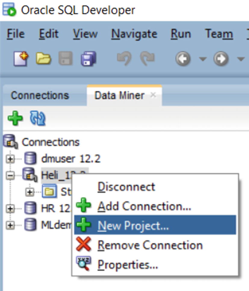
Creating a project in Data Miner
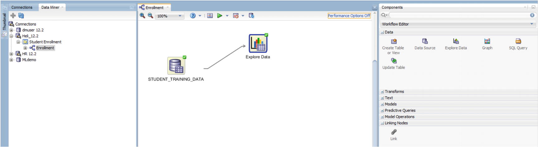
Exploring data using Oracle SQL Developer and Data Miner
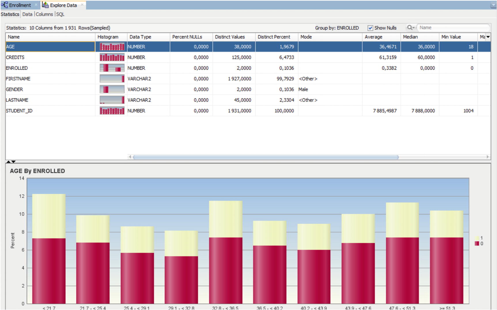
Age by enrolled visualization

Defining the model setting for classification model
Next, run the model. It uses all the algorithms available in the database for classification problems. You can right-click the Class Builder icon and select View Models, View Test Results, or Compare Test Results.
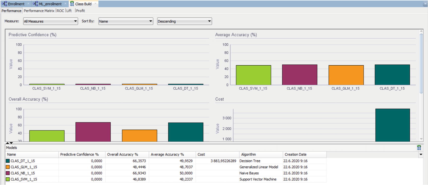
Comparing the different algorithms using Compare Test Results
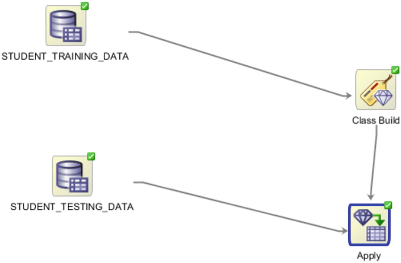
Applying the model to a new data set
Now right-click on the Apply and select View Data to see the predictions. Select Deploy to deploy the model.
Data Miner is very easy to use if you understand the machine learning process. There is no need for any coding. All is done by clicking and drag-and-dropping.
OML Notebooks
In Oracle Cloud, there is a possibility to use an autonomous database. There are two different workloads for an autonomous database: transaction processing (ATP) and data warehousing (ADW). Both of these include one more option to Oracle Machine Learning: OML Notebooks. OML Notebooks are Apache Zeppelin notebooks. Using these notebooks machine learning process is easy to document, and it includes many data visualization functionalities. The OML Notebooks are using the same PL/SQL packages discussed earlier in this chapter. You can read more about OML Notebooks and the autonomous database in Chapters 4, 5, and 6.
Summary
OML4SQL operates in Oracle Database. That means that there is no need to move the data for the machine learning process. It can be processed in the database. Also, the machine learning models are database objects and can be used as any database object. There are PL/SQL packages in the database to prepare and transform the data for machine learning and build and evaluate the machine learning models. Those packages can be used from any interface that allows calling PL/SQL packages. They can also be used with the GUI of Oracle Data Miner plug-in in Oracle SQL Developer or OML Notebooks in OCI.