In the previous chapters so far, we have seen supervised Machine Learning where the target variable or label is known to us, and we try to predict the output based on the input features. Unsupervised Learning is different in a sense that there is no labeled data, and we don’t try to predict any output as such; instead we try to find interesting patterns and come up with groups within the data. The similar values are grouped together.
When we join a new school or college, we come across many new faces and everyone looks so different. We hardly know anyone in the institute, and there are no groups in place initially. Slowly and gradually, we start spending time with other people and the groups start to develop. We interact with a lot of different people and figure out how similar and dissimilar they are to us. A few months down the line, we are almost settled in our own groups of friends. The friends/members within the group have similar attributes/likings/tastes and hence stay together. Clustering is somewhat similar to this approach of forming groups based on sets of attributes that define the groups.
Starting with Clustering
We can apply clustering on any sort of data where we want to form groups of similar observations and use it for better decision making. In the early days, customer segmentation used to be done by a Rule-based approach, which was much of a manual effort and could only use a limited number of variables. For example, if businesses wanted to do customer segmentation, they would consider up to 10 variables such as age, gender, salary, location, etc., and create rules-based segments that still gave reasonable performance; but in today’s scenario that would become highly ineffective. One reason is data availability is in abundance, and the other is dynamic customer behavior. There are thousands of other variables that can be considered to come up with these machine learning driven segments that are more enriched and meaningful.
When we start clustering, each observation is different and doesn’t belong to any group but is based on how similar are the attributes of each observation. We group them in such a way that each group contains the most similar records, and there is as much difference as possible between any two groups. So, how do we measure if two observations are similar or different?
There are multiple approaches to calculate the distance between any two observations. Primarily we represent that any observation is a form of vector that contains values of that observation(A) as shown below.
Age
Salary ($’0000)
Weight (Kgs)
Height(Ft.)
32
8
65
6
Now, suppose we want to calculate the distance of this observation/record from any other observation (B), which also contains similar attributes like those shown below.
Age
Salary ($’000)
Weight (Kgs)
Height(Ft.)
40
15
90
5
We can measure the distance using the Euclidean method, which is straightforward.
It is also known as Cartesian distance. We are trying to calculate the distance of a straight line between any two points; and if the distance between those is points is small, they are more likely to be similar, whereas if the distance is large, they are dissimilar to each other as shown in Figure 8-1.
Figure 8-1
Euclidean Distance based similarity
The Euclidean distance between any two points can be calculated using the formula below:
Dist(A, B)= 27.18
Hence, the Euclidean distance between observations A and B is 27.18. The other techniques to calculate the distance between observations are the following:
1.
Manhattan Distance
2.
Mahalanobis Distance
3.
Minkowski Distances
4.
Chebyshev Distance
5.
Cosine Distance
The aim of clustering is to have minimal intracluster distance and maximum intercluster difference. We can end up with different groups based on the distance approach that we have used to do clustering, and hence it's critical to be sure of opting for the right distance metric that aligns with the business problem. Before going into different clustering techniques, let quickly go over some of the applications of clustering.
Applications
Clustering is used in a variety of use cases these days ranging from customer segmentation to anomaly detection. Businesses widely use machine learning driven clustering for profiling customer and segmentation to create market strategies around these results. Clustering drives a lot of search engines' results by finding similar objects in one cluster and the dissimilar objects far from each other. It recommends the nearest similar result based on a search query
Clustering can be done in multiple ways based on the type of data and business requirement. The most used ones are the K-means and Hierarchical clustering.
K-Means
‘K’ stands for a number of clusters or groups that we want to form in the given dataset. This type of clustering involves deciding the number of clusters in advance. Before looking at how K-means clustering works, let’s get familiar with a couple of terms first.
1.
Centroid
2.
Variance
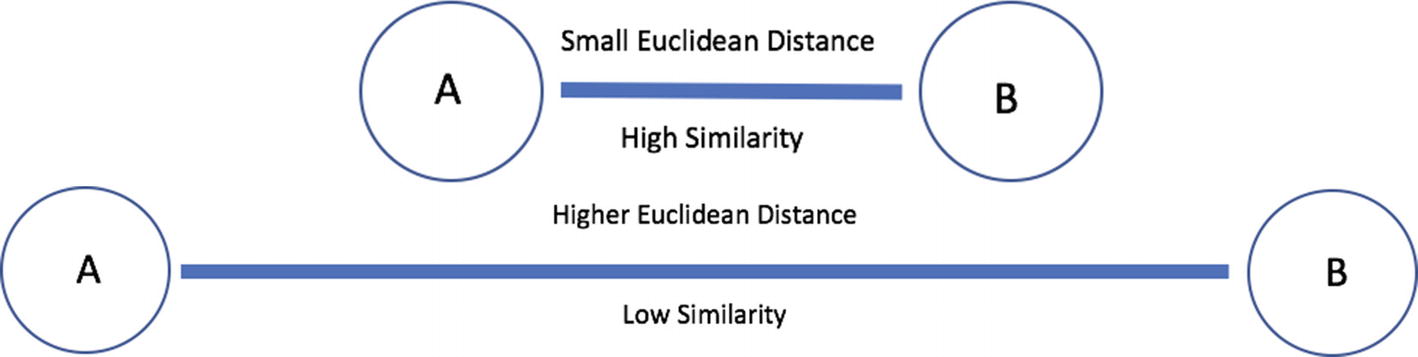
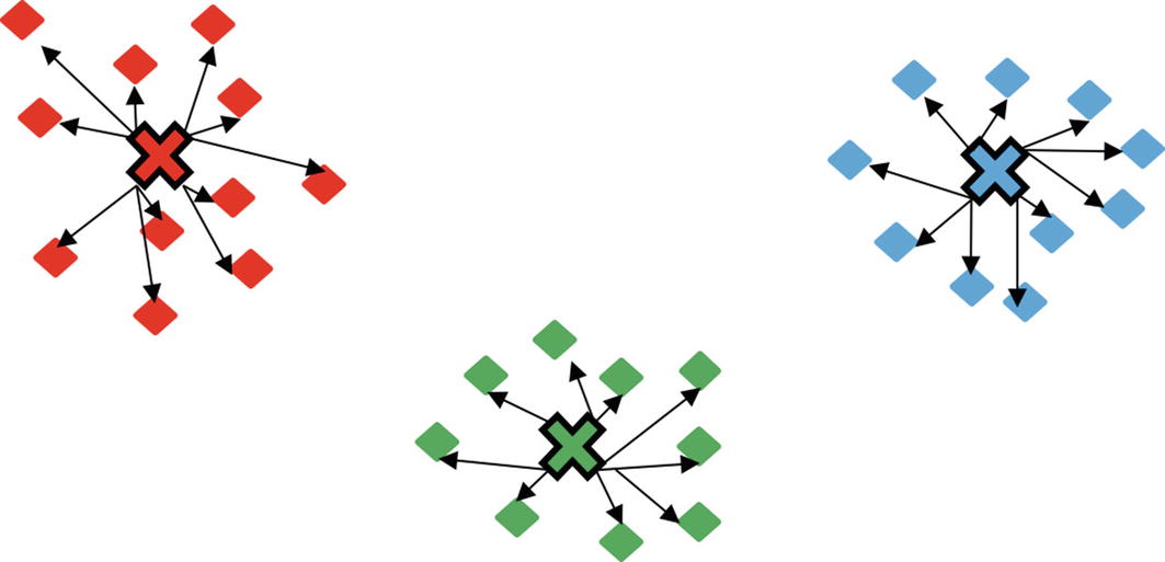
Centroid refers to the center data point at the center of a cluster or a group. It is also the most representative point within the cluster as it’s the utmost equidistant data point from the other points within the cluster. The centroid (represented by a cross) for three random clusters is shown in Figure 8-2.
Figure 8-2
Centroids of clusters
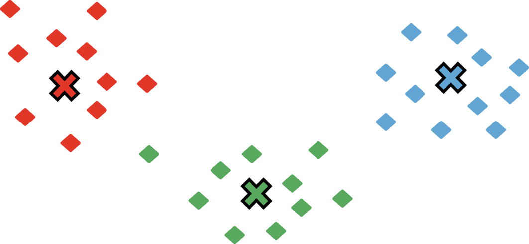
Each cluster or group contains different number of data points that are nearest to the centroid of the cluster. Once the individual data points change clusters, the centroid value of the cluster also changes. The center position within a group is altered, resulting in a new centroid as shown in Figure 8-3.
Figure 8-3
New Centroids of new clusters
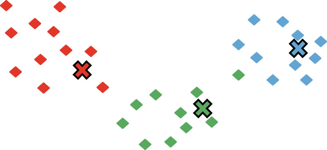
The whole idea of clustering is to minimize intracluster distance, that is, the internal distance of data points from the centroid of cluster and maximize the intercluster distance, that is, between the centroid of two different clusters.
Variance is the total sum of intracluster distances between centroid and data points within that cluster as show in Figure 8-4. The variance keeps on decreasing with an increase in the number of clusters. The more clusters, the less the number of data points within each cluster and hence less variability.
Figure 8-4
Inracluster Distance
K-means clustering is composed of four steps in total to form the internal groups within the dataset. We will consider a sample dataset to understand how a K-means clustering algorithm works. The dataset contains a few users with their age and weight values as shown in Table 8-1. Now we will use K-means clustering to come up with meaningful clusters and understand the algorithm.
Table 8-1
Sample Dataset for K-Means
User ID
Age
Weight
1
18
80
2
40
60
3
35
100
4
20
45
5
45
120
6
32
65
7
17
50
8
55
55
9
60
90
10
90
50
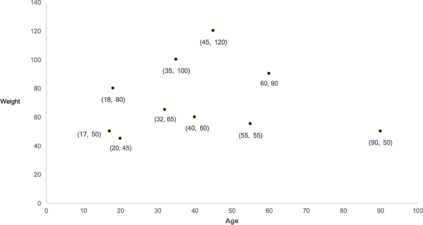
If we plot these users in a two-dimensional space, we can see that no point belongs to any group initially, and our intention is to find clusters (we can try with two or three) within this group of users such that each group contains similar users. Each user is represented by the age and weight as shown in Figure 8-5.
Figure 8-5
Users before clustering
Step I: Decide K
It starts with deciding the number of clusters(K) . Most of the time, we are not sure of the right number of groups at the start, but we can find the best number of clusters using a method called the Elbow method based on variability. For this example, let’s start with K=2 to keep things simple. So, we are looking for two clusters within this sample data.
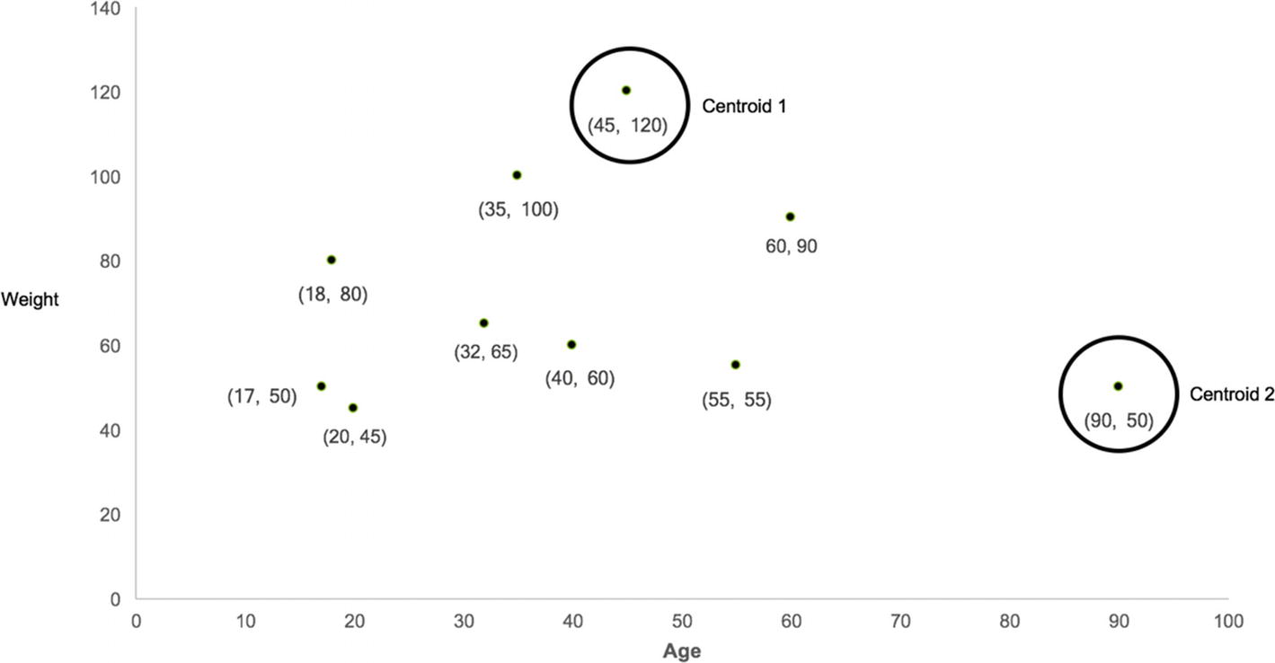
Step 2: Random Initialization of Centroids
The next step is to randomly consider any two of the points to be a centroid of new clusters. These can be chosen randomly, so we select user number 5 and user number 10 as the two centroids on the new clusters as shown in Table 8-2.
Table 8-2
Sample Dataset for K-Means
User ID
Age
Weight
1
18
80
2
40
60
3
35
100
4
20
45
5 (Centroid 1)
45
120
6
32
65
7
17
50
8
55
55
9
60
90
10 (centroid 2)
90
50
The centroids can be represented by weight and age values as shown in Figure 8-6.
Figure 8-6
Random Centroids of two clusters
Step 3: Assigning Cluster Number to each Value
In this step, we calculate the distance of each point from the centroid. In this example, we calculate the Euclidean squared distance of each user from the two centroid points. Based on the distance value, we go ahead and decide which particular cluster the user belongs to (1 or 2). Whichever centroid the user is near to (less distance) would become part of that cluster. The Euclidean squared distance is calculated for each user shown in Table 8-3. The distance of user 5 and user 10 would be zero from respective centroids as they are the same points as centroids.
Table 8-3
Cluster Assignment Based on Distance from Centroids
User ID
Age
Weight
ED* from Centroid 1
ED* from Centroid 2
Cluster
1
18
80
48
78
1
2
40
60
60
51
2
3
35
100
22
74
1
4
20
45
79
70
2
5
45
120
0
83
1
6
32
65
57
60
1
7
17
50
75
73
2
8
55
55
66
35
2
9
60
90
34
50
1
10
90
50
83
0
2
(*Euclidean Distance)
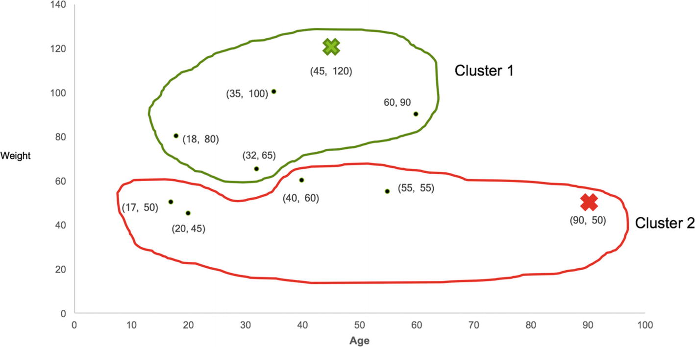
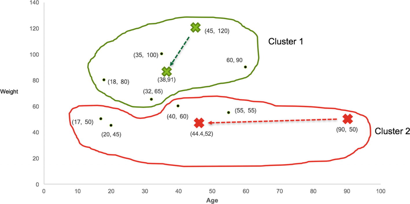
So, as per the distance from centroids, we have allocated each user to either Cluster 1 or Cluster 2. Cluster 1 contains five users and Cluster 2 also contains five users. The initial clusters are shown in Figure 8-7.
Figure 8-7
Initial clusters and centroids
As discussed earlier, the centroids of the clusters are bound to change after inclusion or exclusion of new data points in the cluster. As the earlier centroids (C1, C2) are no longer at the center of clusters, we calculate new centroids in the next step.
Step 4: Calculate New Centroids and Reassign Clusters
The final step in K-means clustering is to calculate the new centroids of clusters and reassign the clusters to each value based on the distance from new centroids. Let’s calculate the new centroid of Cluster 1 and Cluster 2. To calculate the centroid of Cluster 1, we simply take the mean of age and weight for only those values that belong to Cluster 1 as shown in Table 8-4.
Table 8-4
New Centroid Calculation of Cluster 1
User ID
Age
Weight
1
18
80
3
35
100
5
45
120
6
32
65
9
60
90
Mean Value
38
91
The centroid calculation for Cluster 2 is also done in a similar manner and shown in Table 8-5.
Table 8-5
New Centroid calculation of Cluster 2
User ID
Age
Weight
2
40
60
4
20
45
7
17
50
8
55
55
10
90
50
Mean Value
44.4
52
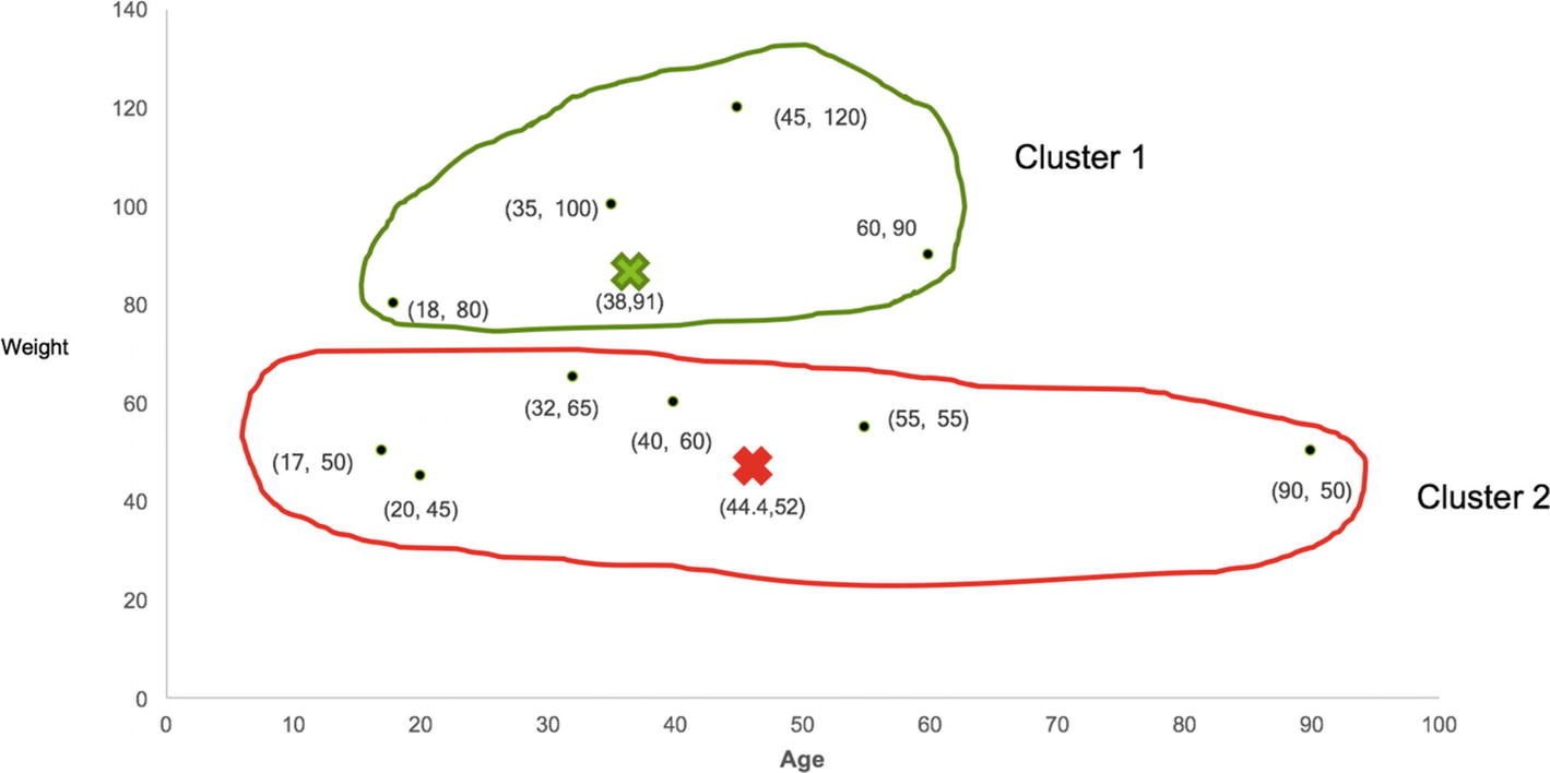
Now we have new centroid values for each cluster represented by a cross as shown in Figure 8-8. The arrow signifies the movement of the centroid within the cluster.
Figure 8-8
New Centroids of both clusters
With centroids of each cluster, we repeat step 3 of calculating the Euclidean squared distance of each user from new centroids and find out the nearest centroid. We then reassign the users to either Cluster 1 or Cluster 2 based on the distance from the centroid. In this case, only one value (User 6) changes its cluster from 1 to 2 as shown in Table 8-6.
Table 8-6
Reallcoation of Clusters
User ID
Age
Weight
ED* from Centroid 1
ED* from Centroid 2
Cluster
1
18
80
23
38
1
2
40
60
31
9
2
3
35
100
9
49
1
4
20
45
49
25
2
5
45
120
30
68
1
6
32
65
27
18
2
7
17
50
46
27
2
8
55
55
40
11
2
9
60
90
22
41
1
10
90
50
66
46
2
Now, Cluster 1 is left with only four users and Cluster 2 contains six users based on the distance from each cluster's centroid as shown in Figure 8-9.
Figure 8-9
Reallocation of clusters
We keep repeating the above steps until there is no more change in cluster allocations. The centroids of new clusters are shown in Table 8-7.
Table 8-7
Calculation of Centroids
User ID
Age
Weight
1
18
80
3
35
100
5
45
120
9
60
90
Mean Value
39.5
97.5
User ID
Age
Weight
2
40
60
4
20
45
6
32
65
7
17
50
8
55
55
10
90
50
Mean Value
42.33
54.17
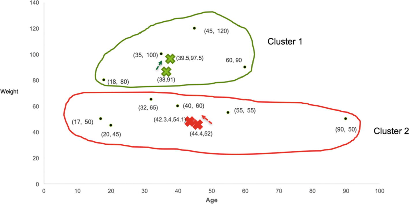
As we go through the steps, the centroid movements keep becoming small, and the values almost become part of that particular cluster as shown in Figure 8-10.
Figure 8-10
Reallocation of clusters
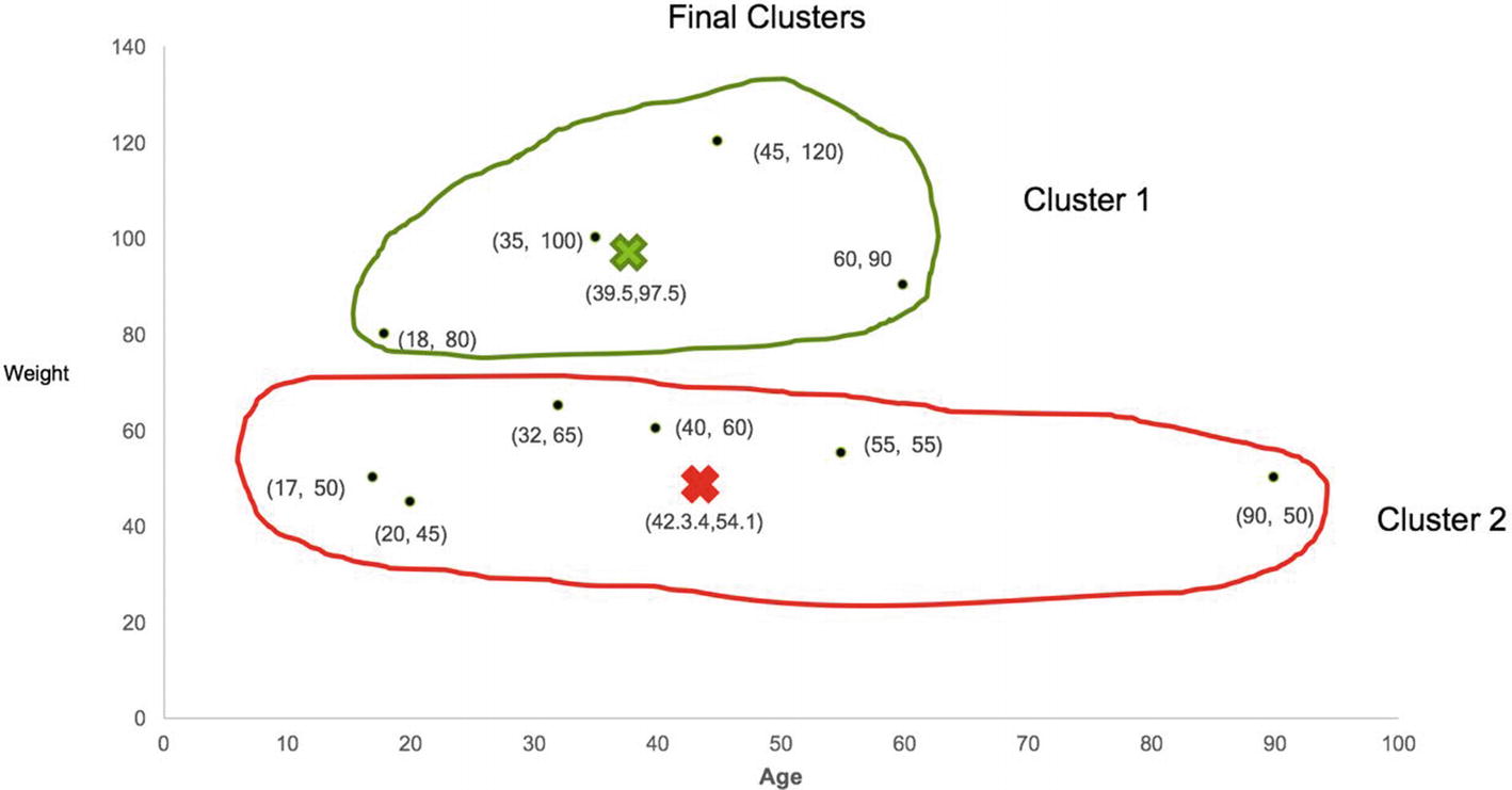
As we can observe, there is no more change in the points even after the change in centroids, which completes the K-means clustering. The results can vary as it’s based on the first set of random centroids. To reproduce the results, we can set the starting points ourselves as well. The final clusters with values are shown in Figure 8-11.
Figure 8-11
Final clusters
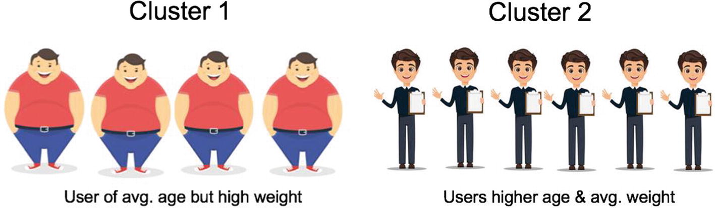
Cluster 1 contains the users that are average on the height attribute but seem to be very high on the weight variable whereas Cluster 2 seems to be grouping those users together who are taller than average but very conscious of their weight as shown in Figure 8-12.
Figure 8-12
Attributes of final clusters
Deciding on Number of Clusters (K)
Selecting an optimal number of clusters is quite tricky most of the time as we need a deep understanding of the dataset and the context of the business problem. Additionally, there is no right or wrong answer when it comes to unsupervised learning. One approach might result in a different number of clusters compared to another approach. We have to try and figure out which approach works the best and if the clusters created are relevant enough for decision making. Each cluster can be represented with a few important attributes that signify or give information about that particular cluster. However, there is a method to pick the best possible number of clusters with a dataset. This method is known as the elbow method.
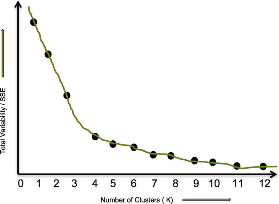
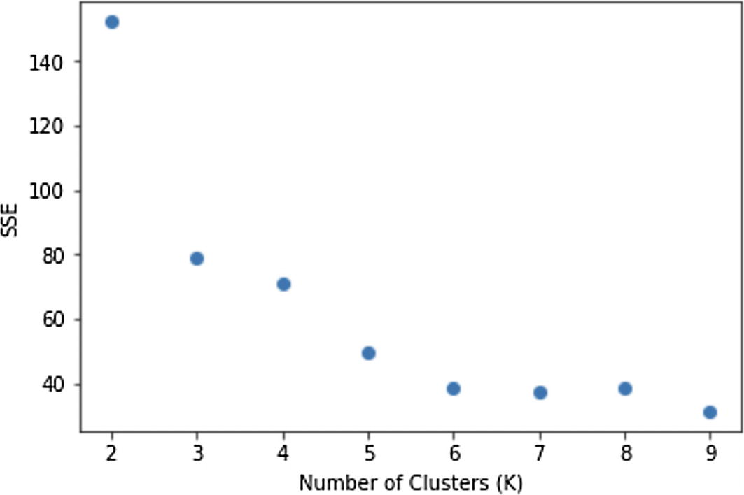
The elbow method helps us to measure the total variance in the data with a number of clusters. The higher the number of clusters, the less the variance would become. If we have an equal number of clusters to the number of records in a dataset, then the variability would be zero because the distance of each point from itself is zero. The variability or SSE (Sum of Squared Errors) along with ‘K’ values is shown in Figure 8-13.
Figure 8-13
Elbow Method
As we can observe, there is sort of elbow formation between K values of 3 and 4. There is a sudden reduction in total variance (intra-cluster difference), and the variance sort of declines very slowly after that. In fact, it flattens after the K=9 value. So, the value of K =3 makes the most sense if we go with the elbow method as it captures the most variability with a lesser number of clusters.
Hierarchical Clustering
This is another type of unsupervised machine learning technique and is different from K-means in the sense that we don’t have to know the number of clusters in advance. There are two types of Hierarchical clustering.
Agglomerative Clustering (Bottom-Up Approach)
Divisive Clustering (Top-Down Approach)
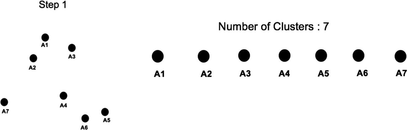
We’ll discuss agglomerative clustering as it is the main type. This starts with the assumption that each data point is a separate cluster and gradually keeps combining the nearest values into the same clusters until all the values become part of one cluster. This is a bottom-up approach that calculates the distance between each cluster and merges the two closest clusters into one. Let’s understand the agglomerative clustering with help of visualization. Let’s say we have seven data points initially (A1–A7), and they need to be grouped into clusters that contain similar values together using agglomerative clustering as shown in Figure 8-14.
Figure 8-14
Each value as individual cluster
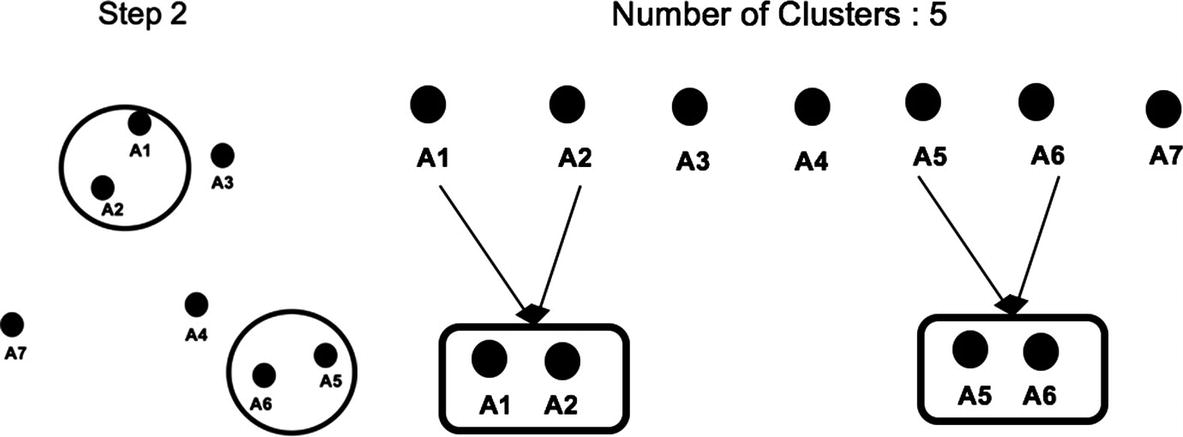
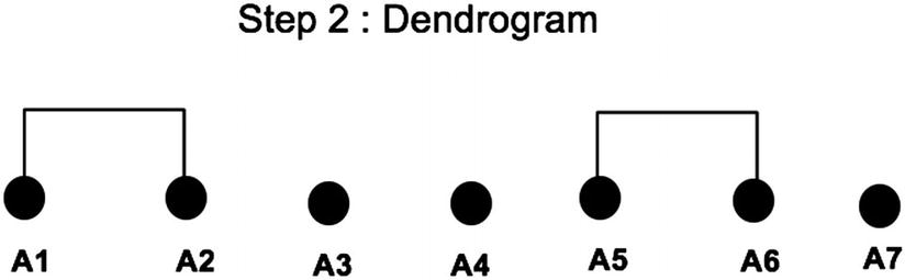
At the initial stage (step 1), each point is treated as an individual cluster. In the next step, the distance between every point is calculated and the nearest points are combined together into a single cluster. In this example, A1 and A2, A5 and A6 are nearest to each other and hence form a single cluster as shown in Figure 8-15.
Figure 8-15
Nearest clusters merged together
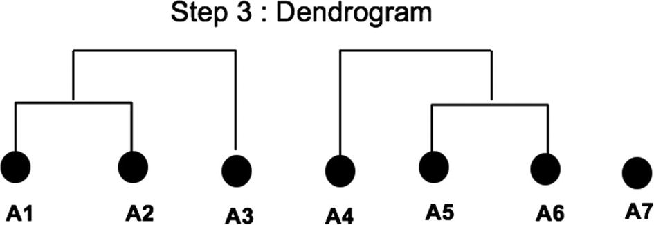
Deciding the most optimal number of clusters while using Hierarchical clustering can be done in multiple ways. One way is to use the elbow method itself and the other option is by making use of something known as a Dendrogram. It is used to visualize the variability between clusters (Euclidean distance). In a Dendrogram, the height of the vertical lines represents the distance between points or clusters and data points listed along the bottom. Each point is plotted on the X-axis and the distance is represented on the Y-axis (length). It is the hierarchical representation of the data points. In this example, the Dendrogram at step 2 looks like the one shown in Figure 8-16.
Figure 8-16
Dendrogram
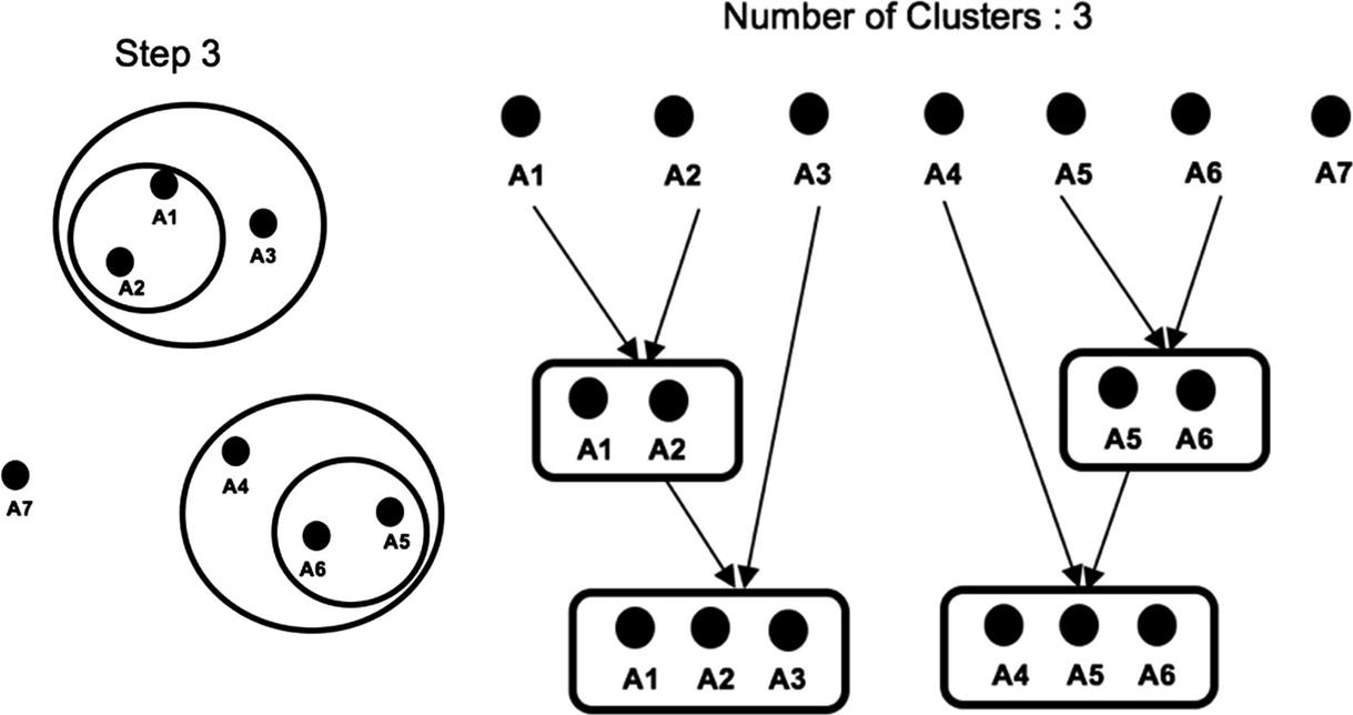
In step 3, the exercise of calculating the distance between clusters is repeated and the nearest clusters are combined into a single cluster. This time A3 gets merged with (A1, A2) and A4 with (A5, A6) as shown in Figure 8-17.
Figure 8-17
Nearest clusters merged together
The Dendrogram after step 3 is shown in Figure 8-18.
Figure 8-18
Dendrogram post step 3
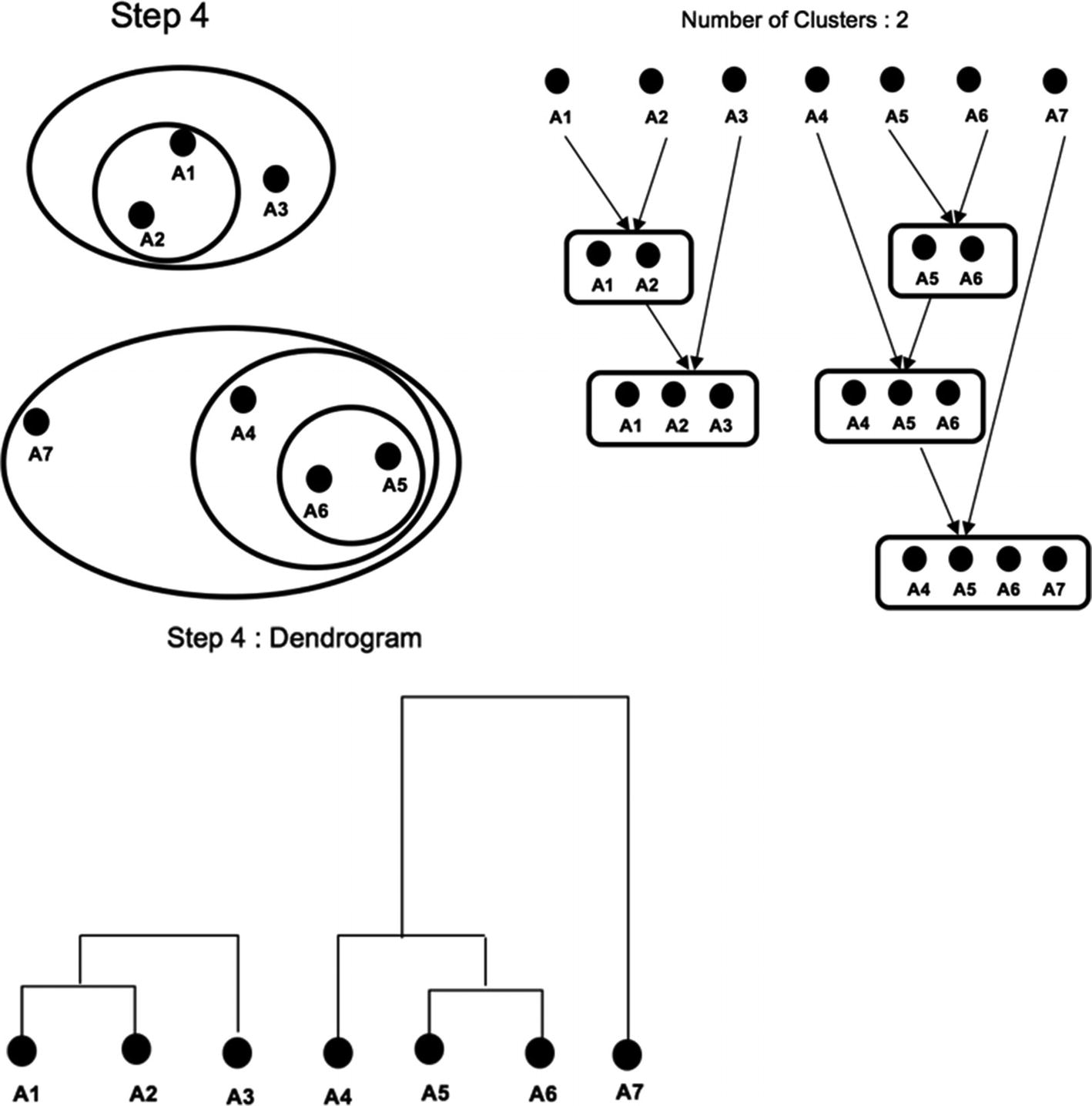
In step 4, the distance between the only remaining point A7 gets calculated and found nearer to Cluster (A4, A5, A6). It is merged with the same cluster as shown in Figure 8-19.
Figure 8-19
Cluster formation
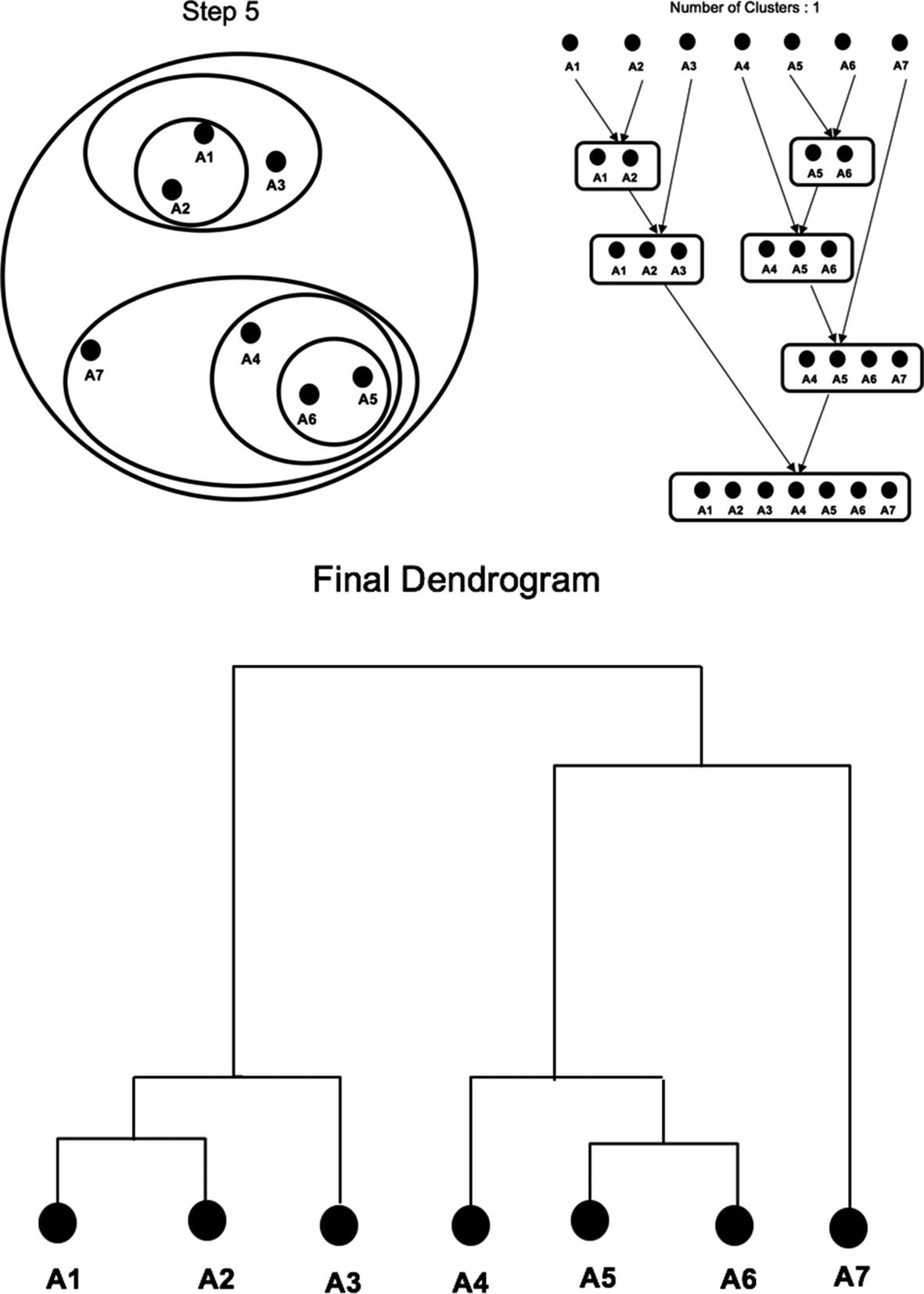
At the last stage (step 5), all the points get combined into a single Cluster (A1, A2, A3, A4, A5, A6, A7) as shown in Figure 8-20.
Figure 8-20
Agglomerative clustering
Sometimes it is difficult to identify the right number of clusters by the Dendrogram as it can become very complicated and difficult to interpret depending on the dataset being used to do clustering. The Hierarchical clustering doesn’t work well on large datasets compared to K-means. Clustering is also very sensitive to the scale of data points, so it's always advised to do data scaling before clustering. There are other types of clustering that can be used to group the similar data points together such as the following:
1.
Gaussian Mixture Model Clustering
2.
Fuzzy C-Means Clustering
But the above methods are beyond the scope of this book. We now jump into using a dataset for building clusters using K-means in PySpark.
Code
This section of the chapter covers K-Means clustering using PySpark and Jupyter Notebook.
Note
The complete dataset along with the code is available for reference on the GitHub repo of this book and executes best on Spark 2.0 and higher versions.
For this exercise, we consider the most standardized open sourced dataset out there – an IRIS dataset to capture the cluster number and compare supervised and unsupervised performance.
Data Info
The dataset that we are going to use for this chapter is the famous open sourced IRIS dataset and contains a total of 150 records with 5 columns (sepal length, sepal width, petal length, petal width, species). There are 50 records for each type of species. We will try to group these into clusters without using the species label information.
Step 1: Create the SparkSession Object
We start Jupyter Notebook and import SparkSession and create a new SparkSession object to use Spark:
We then load and read the dataset within Spark using a dataframe. We have to make sure we have opened PySpark from the same directory folder where the dataset is available or else we have to mention the directory path of the data folder.
In this section, we explore the dataset by viewing it and validating its shape.
[In]:print((df.count(), len(df.columns)))
[Out]: (150,3)
So, the above output confirms the size of our dataset and we can then validate the datatypes of the input values to check if we need to change/cast any columns' datatypes.
[In]: df.printSchema()
[Out]: root
|-- sepal_length: double (nullable = true)
|-- sepal_width: double (nullable = true)
|-- petal_length: double (nullable = true)
|-- petal_width: double (nullable = true)
|-- species: string (nullable = true)
There is a total of five columns out of which four are numerical and the label column is categorical.
So, it confirms that there are an equal number of records for each species available in the dataset
Step 4: Feature Engineering
This is the part where we create a single vector combining all input features by using Spark’s VectorAssembler. It creates only a single feature that captures the input values for that particular row. So, instead of four input columns (we are not considering a label column since it's an unsupervised machine learning technique), it essentially translates it into a single column with four input values in the form of a list.
[In]: from pyspark.ml.linalg import Vector
[In]: from pyspark.ml.feature import VectorAssembler
The final data contains the input vector that can be used to run K-means clustering. Since we need to declare the value of ‘K’ in advance before using K-means, we can use elbow method to figure out the right value of ‘K’. In order to use the elbow method, we run K-means clustering for different values of ‘K’. First, we import K-means from the PySpark library and create an empty list that would capture the variability or SSE (within cluster distance) for each value of K.
[In]:from pyspark.ml.clustering import KMeans
[In]:errors=[]
[In]:
for k in range(2,10):
kmeans = KMeans(featuresCol='features',k=k)
model = kmeans.fit(final_data)
intra_distance = model.computeCost(final_data)
errors.append(intra_distance)
Note
The ‘K’ should have a minimum value of 2 to be able to build clusters.
Now, we can plot the intracluster distance with the number of clusters using numpy and matplotlib.
[In]: import pandas as pd
[In]: import numpy as np
[In]: import matplotlib.pyplot as plt
[In]: cluster_number = range(2,10)
[In]: plt.xlabel('Number of Clusters (K)')
[In]: plt.ylabel('SSE')
[In]: plt.scatter(cluster_number,errors)
[In]: plt.show()
[Out]:
In this case, k=3 seems to be the best number of clusters as we can see a sort of elbow formation between three and four values. We build final clusters using k=3.
K-Means clustering gives us three different clusters based on the IRIS data set. We certainly are making a few of the allocations wrong as only one category has 50 records in the group, and the rest of the categories are mixed up. We can use the transform function to assign the cluster number to the original dataset and use a groupBy function to validate the groupings.
As it can be observed, the setosa species is perfectly grouped along with versicolor, almost being captured in the same cluster, but verginica seems to fall within two different groups. K-means can produce different results every time as it chooses the starting point (centroid) randomly every time. Hence, the results that you might get in you K-means clustering might be totally different from these results unless we use a seed to reproduce the results. The seed ensures the split and the initial centroid values remain consistent throughout the analysis.
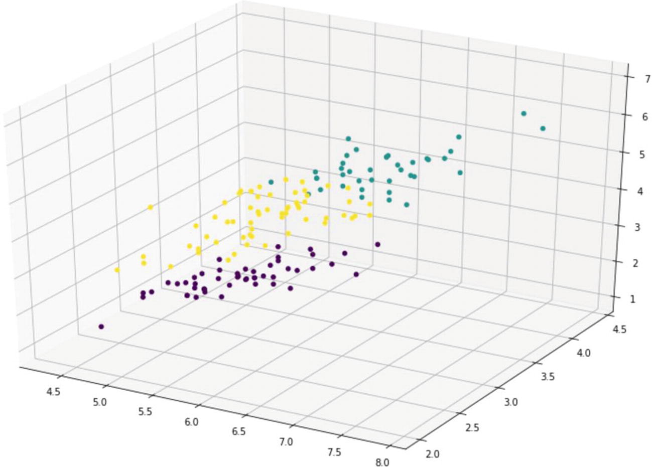
Step 6: Visualization of Clusters
In the final step, we can visualize the new clusters with the help of Python’s matplotlib library. In order to do that, we convert our Spark dataframe into a Pandas dataframe first.
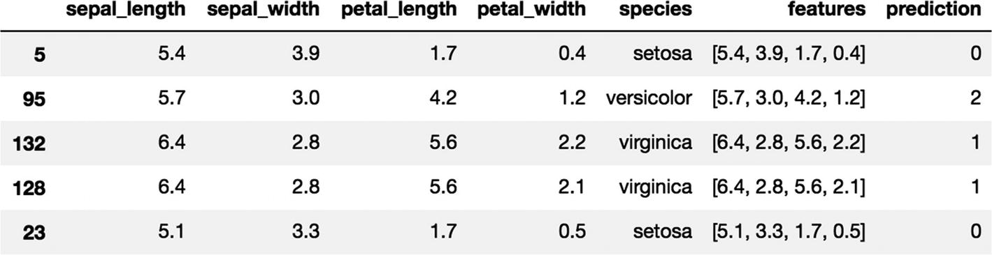
[In]: pandas_df = predictions.toPandas()
[In]: pandas_df.head()
We import the required libraries to plot the third visualization and observe the clusters.
In this chapter, we went over different types of unsupervised machine learning techniques and also built clusters using the K-means algorithms in PySpark. K-Means groups the data points using random centroid initialization whereas Hierarchical clustering focuses on merging entire datapoints into a single cluster. We also covered various techniques to decide the optimal number of clusters like the Elbow method and Dendrogram, which use variance optimization while grouping the data points.