A common trend that can be observed in brick and mortar stores, is that we have salespeople guiding and recommending us relevant products while shopping on the other hand, with online retail platforms, there are zillions of different products available, and we have to navigate ourselves to find the right product. The situation is that users have too many options and choices available, yet they don’t like to invest a lot of time going through the entire catalogue of items. Hence, the role of Recommender Systems (RS) becomes critical for recommending relevant items and driving customer conversion.
Traditional physical stores use planograms to arrange the items in such a way that can increase the visibility of high-selling items and increase revenue whereas online retail stores need to keep it dynamic based on preferences of each individual customer rather than keeping it the same for everyone.
Recommender systems are mainly used for auto-suggesting the right content or product to the right users in a personalized manner to enhance the overall experience. Recommender systems are really powerful in terms of using huge amounts of data and learning to understand the preferences of specific users. Recommendations help users to easily navigate through millions of products or tons of content (articles/videos/movies) and show them the right item/information that they might like or buy. So, in simple terms, RS help discover information on behalf of the users. Now, it depends on the users to decide if RS did a good job at recommendations or not, and they can choose to either select the product/content or discard and move on. Each of the decisions of users (Positive or Negative) helps to retrain the RS on the latest data to be able to give even better recommendations. In this chapter, we will go over how RS work and the different types of techniques used under the hood for making these recommendations. We will also build a recommender system using PySpark.
Recommendations
- 1.
Retail Products
- 2.
Jobs
- 3.
Connections/Friends
- 4.
Movies/Music/Videos/Books/Articles
- 5.
Ads
The “What to Recommend” part totally depends on the context in which RS are used and can help the business to increase revenues by providing the most likely items that users can buy or increasing the engagement by showcasing relevant content at the right time. RS take care of the critical aspect that the product or content that is being recommended should either be something which users might like but would not have discovered on their own. Along with that, RS also need an element of varied recommendations to keep it interesting enough. A few examples of heavy usage of RS by businesses today such as Amazon products, Facebook’s friend suggestions, LinkedIn’s “People you may know,” Netflix’s movie, YouTube’s videos, Spotify’s music, and Coursera’s courses.
- 1.
Increased Revenue
- 2.
Positive Reviews and Ratings by Users
- 3.
Increased Engagement
For the other verticals such as ads recommendations and other content recommendation, RS help immensely to help them find the right thing for users and hence increases adoption and subscriptions. Without RS, recommending online content to millions of users in a personalized manner or offering generic content to each user can be incredibly off target and lead to negative impacts on users.
- 1.
Popularity Based RS
- 2.
Content Based RS
- 3.
Collaborative Filtering based RS
- 4.
Hybrid RS
- 5.
Association Rule Mining based RS
We will briefly go over each one of these except for the last item, that is, Association Rule Mining based RS as it’s out of the scope of this book.
Popularity Based RS
- 1.
No. of times downloaded
- 2.
No. of times bought
- 3.
No. of times viewed
- 4.
Highest rated
- 5.
No. of times shared
- 6.
No. of times liked
This kind of RS directly recommends the best-selling or most watched/bought items to the customers and hence increases the chances of customer conversion. The limitation of this RS is that it is not hyper-personalized.
Content Based RS
Movie ID | Horror | Art | Comedy | Action | Drama | Commercial |
|---|---|---|---|---|---|---|
2310 | 0.01 | 0.3 | 0.8 | 0.0 | 0.5 | 0.9 |
Movie Data
Movie ID | Horror | Art | Comedy | Action | Drama | Commercial |
|---|---|---|---|---|---|---|
2310 | 0.01 | 0.3 | 0.8 | 0.0 | 0.5 | 0.9 |
2631 | 0.0 | 0.45 | 0.8 | 0.0 | 0.5 | 0.65 |
2444 | 0.2 | 0.0 | 0.8 | 0.0 | 0.5 | 0.7 |
2974 | 0.6 | 0.3 | 0.0 | 0.6 | 0.5 | 0.3 |
2151 | 0.9 | 0.2 | 0.0 | 0.7 | 0.5 | 0.9 |
2876 | 0.0 | 0.3 | 0.8 | 0.0 | 0.5 | 0.9 |
2345 | 0.0 | 0.3 | 0.8 | 0.0 | 0.5 | 0.9 |
2309 | 0.7 | 0.0 | 0.0 | 0.8 | 0.4 | 0.5 |
2366 | 0.1 | 0.15 | 0.8 | 0.0 | 0.5 | 0.6 |
2388 | 0.0 | 0.3 | 0.85 | 0.0 | 0.8 | 0.9 |
User Profile
User ID | Horror | Art | Comedy | Action | Drama | Commercial |
|---|---|---|---|---|---|---|
1A92 | 0.251 | 0.23 | 0.565 | 0.21 | 0.52 | 0.725 |
This approach to create the user profile is one of the most baseline ones, and there are other sophisticated ways to create more enriched user profiles such as normalized values, weighted values, etc. The next step is to recommend the items (movies) that this user might like based on the earlier preferences. So, the similarity score between the user profile and item profile is calculated and ranked accordingly. The more the similarity score, the higher the chances of liking the movie by the user. There are a couple of ways by which the similarity score can be calculated.
Euclidean Distance

The higher the distance value, the less similar are the two vectors. Therefore, the distance between the user profile and all other items are calculated and ranked in decreasing order. The top few items are recommended to the user in this manner.
Cosine Similarity
Another way to calculate a similarity score between the user and item profile is cosine similarity. Instead of distance, it measures the angle between two vectors (user profile vector and item profile vector). The smaller the angle between both vectors, the more similar they are to each other. The cosine similarity can be found out using the formula below:
sim(x,y)=cos(θ)= x*y / |x|*|y|
Let’s go over some of the pros and cons of Content based RS.
- 1.
Content based RC works independently of other users’ data and hence can be applied to an individual’s historical data.
- 2.
The rationale behind RC can be easily understood as the recommendations are based on the similarity score between the User Profile and Item Profile.
- 3.
New and unknown items can also be recommended to users just based on historical interests and preferences of users.
- 1.
Item profile can be biased and might not reflect exact attribute values and might lead to incorrect recommendations.
- 2.
Recommendations entirely depend on the history of the user and can only recommend items that are like the historically watched/liked items and do not take into consideration the new interests or liking of the visitor.
Collaborative Filtering Based RS
- 1.
Which movie to watch
- 2.
Which book to read
- 3.
Which restaurant to go to
- 4.
Which place to travel to
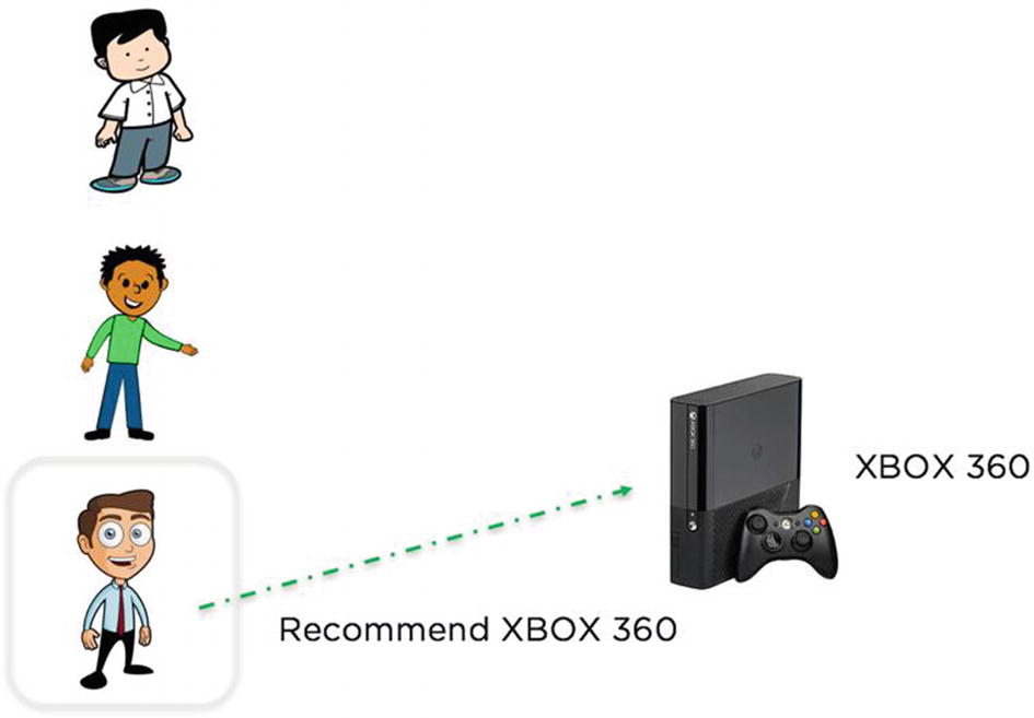
We ask our friends, right! We ask for recommendations from people who are similar to us in some ways and have same tastes and likings as ours. Our interests match in some areas and so we trust their recommendations. These people can be our family members, friends, colleagues, relatives, or community members. In real life, it’s easy to know who are the people falling in this circle, but when it comes to online recommendations, the key task in collaborative filtering is to find the users who are most similar to you. Each user can be represented by a vector that contains the feedback value of a user item interaction. Let’s understand the user item matrix first to understand the CF approach.
User Item Matrix
User Item Matrix
User ID | Item 1 | Item 2 | Item 3 | Item 4 | Item 5 | Item n |
|---|---|---|---|---|---|---|
14SD | 1 | 4 | 5 | |||
26BB | 3 | 3 | 1 | |||
24DG | 1 | 4 | 1 | 5 | 2 | |
59YU | 2 | 5 | ||||
21HT | 3 | 2 | 1 | 2 | 5 | |
68BC | 1 | 5 | ||||
26DF | 1 | 4 | 3 | 3 | ||
25TR | 1 | 4 | 5 | |||
33XF | 5 | 5 | 5 | 1 | 5 | 5 |
73QS | 1 | 3 | 1 |
As you can observe, the user item matrix is generally very sparse as there are millions of items, and each user doesn’t interact with every item; so the matrix contains a lot of null values. The values in the matrix are generally feedback values deduced based upon the interaction of the user with that particular item. There are two types of feedback that can be considered in the UI matrix.
Explicit Feedback
- 1.
Rating on 1–5 scale
- 2.
Simple rating item on recommending to others (Yes or No or never)
- 3.
Liked the Item (Yes or No)
The Explicit feedback data contains very limited amounts of data points as a very small percentage of users take out the time to give ratings even after buying or using the item. A perfect example can be of a movie, as very few users give the ratings even after watching it. Hence, building RS solely on explicit feedback data can put us in a tricky situation, although the data itself is less noisy but sometimes not enough to build RS.
Implicit Feedback
This kind of feedback is not direct and mostly inferred from the activities of the user on the online platform and is based on interactions with items. For example, if user has bought the item, added it to the cart, viewed, and spent a great deal of time on looking at the information about the item, this indicates that the user has a higher amount of interest in the item. Implicit feedback values are easy to collect, and plenty of data points are available for each user as they navigate their way through the online platform. The challenges with implicit feedback are that it contains a lot of noisy data and therefore doesn’t add too much value in the recommendations.
- 1.
Nearest Neighbors based CF
- 2.
Latent Factor based CF
Nearest Neighbors Based CF
User Item Matrix
User ID | Item 1 | Item 2 | Item 3 | Item 4 | Item 5 | Item n |
|---|---|---|---|---|---|---|
14SD | 1 | 4 | 5 | |||
26BB | 3 | 3 | 1 | |||
24DG | 1 | 4 | 1 | 5 | 2 | |
59YU | 2 | 5 | ||||
26DF | 1 | 4 | 3 | 3 |
Let’s say we have in total five users and we want to find the two nearest neighbors to the active user (14SD). The Jaccard similarity can be found out using
sim(x,y)=|Rx ∩ Ry|/ | Rx ∪ Ry|
So, this is the number of items that any two users have rated in common divided by the total number of items that both users have rated:
sim (user1, user2) = 1 / 5 = 0.2 since they have rated only Item 2 in common).
User Similarity Score
User ID | Similarity Score |
|---|---|
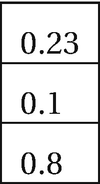
14SD | 1 |
26BB | 0.2 |
24DG | 0.6 |
59YU | 0.677 |
26DF | 0.75 |
So, according to Jaccard similarity the top two nearest neighbors are the fourth and fifth users. There is a major issue with this approach, though, because the Jaccard similarity doesn’t consider the feedback value while calculating the similarity score and only considers the common items rated. So, there could be a possibility that users might have rated many items in common, but one might have rated them high and the other might have rated them low. The Jaccard similarity score still might end up with a high score for both users, which is counterintuitive. In the above example, it is clearly evident that the active user is most similar to the third user (24DG) as they have the exact same ratings for three common items whereas the third user doesn’t even appear in the top two nearest neighbors. Hence, we can opt for other metrics to calculate the k-nearest neighbors.
Missing Values
- 1.
Replace the missing value with 0s.
- 2.
Replace the missing values with average ratings of the user.
- 1.
User based CF
- 2.
Item based CF
The only difference between both RS is that in user based we find k-nearest users, and in item based CF we find k-nearest items to be recommended to users. We will see how recommendations work in user based RS.

Active User and Nearest Neighbors

All users like a item

Nearest Neighbors also like the other item
Active User Recommendation
Latent Factor Based CF
Latent Factor Calculation
1 | 2 | 3 | 5 |
|---|---|---|---|
2 | 4 | 8 | 12 |
3 | 6 | 7 | 13 |
then we can write all the column values as linear combinations of the first and third columns (A1 and A3).
A1 = 1 * A1 + 0 * A3
A2 = 2 * A1 + 0 * A3
A3 = 0 * A1 + 1 * A3
A4 = 2 * A1 + 1 * A3
Now we can create the two small rank matrices in such a way that the product between those two would return the original matrix A.
1 | 3 |
|---|---|
2 | 8 |
3 | 7 |
1 | 2 | 0 | 2 |
|---|---|---|---|
0 | 0 | 1 | 1 |
X contains columns values of A1 and A3 and Y contains the coefficients of linear combinations.
The dot product between X and Y results back into matrix ‘A’ (original matrix)
- 1.
Users latent factor matrix
- 2.
Items latent factor matrix

The user latent factor matrix contains all the users mapped to these latent factors, and similarly the item latent factor matrix contains all items in columns mapped to each of the latent factors. The process of finding these latent factors is done using machine learning optimization techniques such as Alternating Least squares. The user item matrix is decomposed into latent factor matrices in such a way that the user rating for any item is the product between a user’s latent factor value and the item latent factor value. The main objective is to minimize the total sum of squared errors over the entire user item matrix ratings and predicted item ratings. For example, the predicted rating of the second user (26BB) for Item 2 would be
Rating (user2, item2) =

There would be some amount of error on each of the predicted ratings, and hence the cost function becomes the overall sum of squared errors between predicted ratings and actual ratings. Training the recommendation model includes learning these latent factors in such a way that it minimizes the SSE for overall ratings. We can use the ALS method to find the lowest SSE. The way ALS works is that it fixes first the user latent factor values and tries to vary the item latent factor values such that the overall SSE reduces. In the next step, the item latent factor values are kept fixed, and user latent factor values are updated to further reduce the SSE. This keeps alternating between the user matrix and item matrix until there can be no more reduction in SSE.
- 1.
Content information of the item is not required, and recommendations can be made based on valuable user item interactions.
- 2.
Personalizing experience based on other users.
- 1.
Cold Start Problem: If the user has no historical data of item interactions. then RC cannot predict the k-nearest neighbors for the new user and cannot make recommendations.
- 2.
Missing values: Since the items are huge in number and very few users interact with all the items, some items are never rated by users and can’t be recommended.
- 3.
Cannot recommend new or unrated items: If the item is new and yet to be seen by the user, it can’t be recommended to existing users until other users interact with it.
- 4.
Poor Accuracy: It doesn’t perform that well as many components keep changing such as interests of users, limited shelf life of items, and very few ratings of items.
Hybrid Recommender Systems

Combining Recommendations

Hybrid Recommendations
Hybrid recommendations also include using other types of recommendations such as demographic based and knowledge based to enhance the performance of its recommendations. Hybrid RS have become integral parts of various businesses to help their users consume the right content, therefore deriving a lot of value.
Code
This section of the chapter focuses on building an RS from scratch using the ALS method in PySpark and Jupyter Notebook.
Note
The complete dataset along with the code is available for reference on the GitHub repo of this book and executes best on Spark 2.0 and higher versions.
Let’s build a recommender model using Spark’s MLlib library and predict the rating of an item for any given user.
Data Info
The dataset that we are going to use for this chapter is a subset from a famous open sourced movie lens dataset and contains a total of 0.1 million records with three columns (User_Id,title,rating). We will train our recommender model using 75% of the data and test it on the rest of the 25% user ratings.
Step 1: Create the SparkSession Object
Step 2: Read the Dataset
Step 3: Exploratory Data Analysis


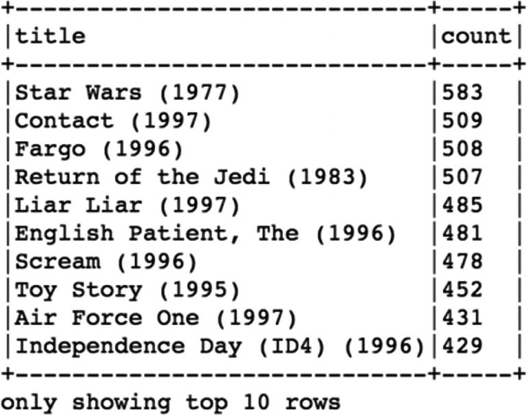
The movie with highest number of ratings is Star Wars (1977) and has been rated 583 times, and each movie has been rated by at least by 1 user.
Step 4: Feature Engineering


Step 5: Splitting the Dataset
Step 6: Build and Train Recommender Model
Step 7: Predictions and Evaluation on Test Data

The RMSE is not very high; we are making an error of one point in the actual rating and predicted rating. This can be improved further by tuning the model parameters and using the hybrid approach.
Step 8: Recommend Top Movies That Active User Might Like


So, the recommendations for the userId (85) are Boys, Les (1997) and Faust (1994). This can be nicely wrapped in a single function that executes the above steps in sequence and generates recommendations for active users. The complete code is available on the GitHub repo with this function built in.
Conclusion
In this chapter, we went over various types of recommendation models along with the strengths and limitations of each. We then created a collaborative filtering based recommender system in PySpark using the ALS method to recommend movies to the users.