This chapter covers

• Defining reinforcement learning
• Implementing reinforcement learning

Humans learn from experiences (or at least should ). You didn’t get so charming by accident. Years of positive compliments as well as negative criticism have all helped shape who you are today. This chapter is about designing a machine-learning system driven by criticisms and rewards.

You learn what makes people happy, for example, by interacting with friends, family members, or even strangers, and you figure out how to ride a bike by trying out various muscle movements until riding clicks. When you perform actions, you’re sometimes rewarded immediately. Finding a good restaurant nearby might yield instant gratification, for example. At other times, the reward doesn’t appear right away; you might have to travel a long distance to find an exceptional place to eat. Reinforcement learning is about choosing the right actions, given any state—such as in figure 13.1, which shows a person making decisions to arrive at their destination.

Figure 13.1 A person navigating to reach a destination in the midst of traffic and unexpected situations is a problem setup for reinforcement learning.

Moreover, suppose that on your drive from home to work, you always choose the same route. But one day, your curiosity takes over, and you decide to try a different path in the hope of shortening your commute. This dilemma—trying new routes or sticking to the best-known route—is an example of exploration versus exploitation.

Note Why is the trade-off between trying new things and sticking with old ones called exploration versus exploitation? Exploration makes sense, but you can think of exploitation as exploiting your knowledge of the status quo by sticking with what you know.

All these examples can be unified under a general formulation: performing an action in a scenario can yield a reward. A more technical term for scenario is state. And we call the collection of all possible states a state space. Performing an action causes the state to change. This shouldn’t be too unfamiliar to you if you remember chapters 9 and 10, which deal with hidden Markov models (HMMs). You transitioned from state to state in those chapters based on observations. But what series of actions yields the highest expected rewards?

13.1 Formal notions

Whereas supervised and unsupervised learning appear at opposite ends of the spectrum, reinforcement learning (RL) exists somewhere in the middle. It’s not supervised learning, because the training data comes from the algorithm deciding between exploration and exploitation. And it’s not unsupervised, because the algorithm receives feedback from the environment. As long as you’re in a situation in which performing an action in a state produces a reward, you can use reinforcement learning to discover a good sequence of actions to take to maximize expected rewards.

You may notice that reinforcement-learning lingo involves anthropomorphizing the algorithm into taking actions in situations to receive rewards. The algorithm is often referred to as an agent that acts with the environment. It shouldn’t be a surprise that much of reinforcement-learning theory is applied in robotics. Figure 13.2 demonstrates the interplay among states, actions, and rewards.

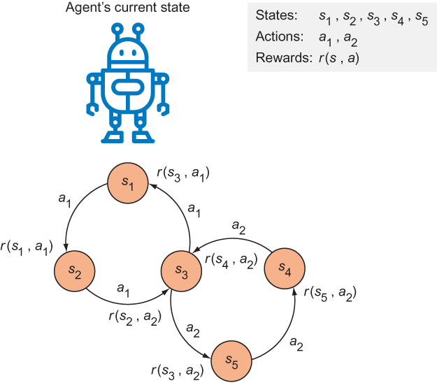
Figure 13.2 Actions are represented by arrows, and states are represented by circles. Performing an action on a state produces a reward. If you start at state s1, you can perform action a1 to obtain a reward r(s1, a1).

A robot performs actions to change states. But how does it decide which action to take? Section 13.1.1 introduces a new concept to answer this question.

13.1.1 Policy

Everyone cleans their room differently. Some people start by making their bed. I prefer cleaning my room clockwise so I don’t miss a corner. Have you ever seen a robotic vacuum cleaner, such as a Roomba? Someone programmed a strategy the robot can follow to clean any room. In reinforcement-learning lingo, the way that an agent decides which action to take is a policy: the set of actions that determines the next state (figure 13.3).

Figure 13.3 A policy suggests which action to take, given a state.

The goal of reinforcement learning is to discover a good policy. A common way to create that policy is to observe the long-term consequences of actions at each state. The reward is the measure of the outcome of taking an action. The best possible policy is called the optimal policy, which is the Holy Grail of reinforcement learning. The optimal policy tells you the optimal action, given any state—but as in real life, it may not provide the highest reward at the moment.

If you measure the reward by looking at the immediate consequence—the state of things after taking the action—it’s easy to calculate. This strategy is called the greedy strategy. But it’s not always a good idea to “greedily” choose the action that provides the best immediate reward. When you’re cleaning your room, for example, you might make your bed first, because the room looks neater with the bed made. But if another goal is to wash your sheets, making the bed first may not be the best overall strategy. You need to look at the results of the next few actions and the eventual end state to come up with the optimal approach. Similarly, in chess, grabbing your opponent’s queen may maximize the points for the pieces on the board—but if it puts you in checkmate five moves later, it isn’t the best possible move.

You can also choose an action arbitrarily, which is a random policy. If you come up with a policy to solve a reinforcement-learning problem, it’s often a good idea to double-check that your learned policy performs better than both the random and greedy policies, which are often called a baseline.

13.1.2 Utility

The long-term reward is called a utility. If you know the utility of performing an action at a state, learning the policy is easy with reinforcement learning. To decide which action to take, you select the action that produces the highest utility. The hard part, as you might have guessed, is uncovering these utility values.

The utility of performing an action (a) at a state (s) is written as a function Q(s, a), called the utility function, shown in figure 13.4.

Figure 13.4 Given a state and the action taken, applying a utility function Q predicts the expected and the total rewards: the immediate reward (next state) plus rewards gained later by following an optimal policy.

An elegant way to calculate the utility of a particular state-action pair (s, a) is to recursively consider the utilities of future actions. The utility of your current action is influenced not only by the immediate reward, but also by the next best action, as shown in the following formula. In the formula, s' is the next state, and a' denotes the next action. The reward of taking action a in state s is denoted by r (s, a):

Q(s, a ) = r (s, a) + γmax Q(s', a')

Here, γ is a hyperparameter that you get to choose, called the discount factor. If γ is 0, the agent chooses the action that maximizes the immediate reward. Higher values of γ will make the agent put more importance on considering long-term consequences. You can read the formula as “the value of this action is the immediate reward provided by taking this action, added to the discount factor times the best thing that can happen after that.”

Looking to future rewards is one type of hyperparameter you can play with, but there’s another. In some applications of reinforcement learning, newly available information might be more important than historical records, or vice versa. If a robot is expected to learn to solve tasks quickly but not necessarily optimally, you might want to set a faster learning rate. Or if a robot is allowed more time to explore and exploit, you might tune down the learning rate. Let’s call the learning rate α, and change the utility function as follows (noting that when α = 1, the equations are identical):

Q(s, a) ← Q(s, a) + α ( r(s, a) + γmax Q(s', a') – Q(s, a))

Reinforcement learning can be solved if you know the Q-function: Q(s, a). Conveniently for us, neural networks (chapters 11 and 12) approximate functions, given enough training data. TensorFlow is the perfect tool to deal with neural networks because it comes with many essential algorithms that simplify neural-network implementation.

13.2 Applying reinforcement learning

Application of reinforcement learning requires defining a way to retrieve rewards after an action is taken from a state. A stock-market trader fits these requirements easily, because buying and selling a stock changes the state of the trader (cash on hand), and each action generates a reward (or loss).

The states in this situation are a vector containing information about the current budget, the current number of stocks, and a recent history of stock prices (the last 200 stock prices). Each state is a 202-dimensional vector.

For simplicity, the only three actions are buy, sell, and hold:

• Buying a stock at the current stock price decreases the budget while incrementing the current stock count.

• Selling a stock trades it in for money at the current share price.

• Holding does neither thing. This action waits a single time period and yields no reward.

Figure 13.5 demonstrates one possible policy, given stock market data.

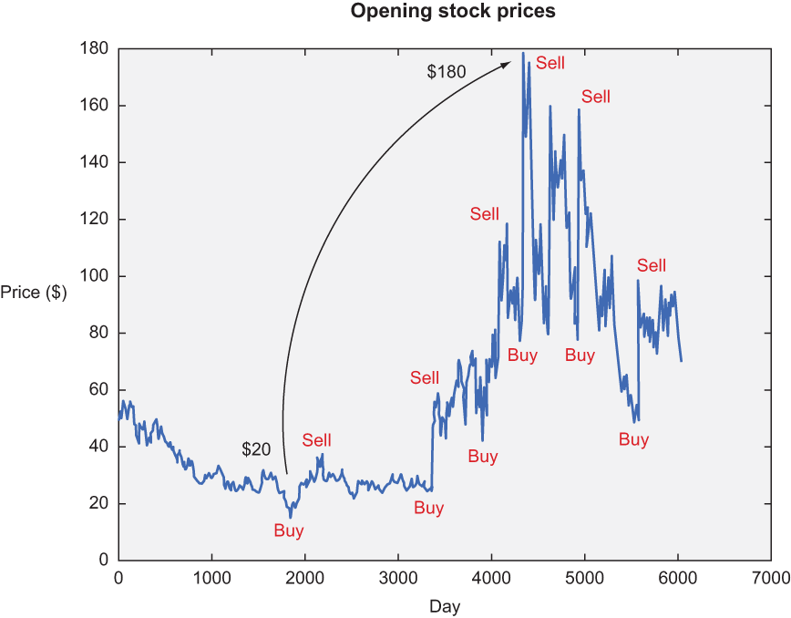
Figure 13.5 Ideally, our algorithm should buy low and sell high. Doing so once, as shown here, might yield a reward of around $160. But the real profit rolls in when you buy and sell more frequently. Have you ever heard the term high-frequency trading? This type of trading involves buying low and selling high as frequently as possible to maximize profits within a given period.

The goal is to learn a policy that gains the maximum net worth from trading in a stock market. Wouldn’t that be cool? Let’s do it!

13.3 Implementing reinforcement learning

To gather stock prices, you’ll use the ystockquote library in Python. You can install it by using pip or follow the official guide (https://github.com/cgoldberg/ystockquote). The command to install it with pip is as follows:

$ pip install ystockquote

With that library installed, let’s import all the relevant libraries (listing 13.1).

Listing 13.1 Importing relevant libraries

import ystockquote                      ❶
from matplotlib import pyplot as plt    ❷
import numpy as np                      ❸
import tensorflow as tf                 ❸
import random

❶ For obtaining stock-price raw data

❷ For plotting stock prices

❸ For numeric manipulation and machine learning

Create a helper function to get stock prices by using the ystockquote library. The library requires three pieces of information: share symbol, start date, and end date. When you pick each of the three values, you’ll get a list of numbers representing the share prices in that period by day.

If you choose start and end dates that are too far apart, fetching that data will take some time. It might be a good idea to save (cache) the data to disk so that you can load it locally next time. Listing 13.2 shows to use the library and cache the data.

Listing 13.2 Helper function to get prices

def get_prices(share_symbol, start_date, end_date,
               cache_filename='stock_prices.npy', force=False):
    try:                                                              ❶
        if force:
            raise IOError
        else:
            stock_prices = np.load(cache_filename)
    except IOError:
        stock_hist = ystockquote.get_historical_prices(share_symbol,  ❷
        ➥ start_date, end_date)                                      ❷
        stock_prices = []
        for day in sorted(stock_hist.keys()):                         ❸
            stock_val = stock_hist[day]['Open']
            stock_prices.append(stock_val)            
        stock_prices = np.asarray(stock_prices)
        np.save(cache_filename, stock_prices)                         ❹
        
    return stock_prices.astype(float) 

❶ Tries to load the data from file if it has already been computed

❷ Retrieves stock prices from the library

❸ Extracts only relevant info from the raw data

❹ Caches the result

As a sanity check, it’s a good idea to visualize the stock-price data. Create a plot, and save it to disk (listing 13.3).

Listing 13.3 Helper function to plot the stock prices

def plot_prices(prices):
    plt.title('Opening stock prices')
    plt.xlabel('day')
    plt.ylabel('price ($)')
    plt.plot(prices)
    plt.savefig('prices.png')
    plt.show()

You can grab some data and visualize it by using listing 13.4.

Listing 13.4 Getting data and visualizing it

if __name__ == '__main__':
  prices = get_prices('MSFT', '1992-07-22', '2016-07-22', force=True)
  plot_prices(prices)

Figure 13.6 shows the chart produced by running listing 13.4.

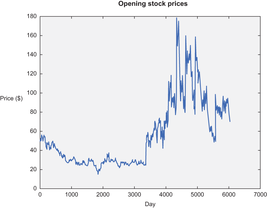
Figure 13.6 This chart summarizes the opening stock prices of Microsoft (MSFT) from July 22, 1992, to July 22, 2016. Wouldn’t it have been nice to buy around day 3,000 and sell around day 5,000? Let’s see whether our code can learn to buy, sell, and hold to make optimal gain.

Most reinforcement-learning algorithms follow similar implementation patterns. As a result, it’s a good idea to create a class with the relevant methods to reference later, such as an abstract class or interface. See listing 13.5 for an example and figure 13.7 for an illustration. Reinforcement learning needs two well-defined operations: how to select an action and how to improve the utility Q-function.

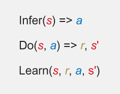
Figure 13.7 Most reinforcement-learning algorithms boil down to three main steps: infer, do, and learn. During the first step, the algorithm selects the best action (a), given a state (s), using the knowledge it has so far. Next, it does the action to find out the reward (r) as well as the next state (s'). Then it improves its understanding of the world by using the newly acquired knowledge (s, r, a, s').

Listing 13.5 Defining a superclass for all decision policies

class DecisionPolicy:
    def select_action(self, current_state):                  ❶
        pass
 
    def update_q(self, state, action, reward, next_state):   ❷
        pass

❶ Given a state, the decision policy will calculate the next action to take.

❷ Improves the Q-function from a new experience of taking an action

Next, let’s inherit from this superclass to implement a policy in which decisions are made at random, otherwise known as a random decision policy. You need to define only the select_action method, which randomly picks an action without even looking at the state. Listing 13.6 shows how to implement it.

Listing 13.6 Implementing a random decision policy

class RandomDecisionPolicy(DecisionPolicy):     ❶
    def __init__(self, actions):
        self.actions = actions
 
    def select_action(self, current_state):     ❷
        action = random.choice(self.actions)
        return action

❶ Inherits from DecisionPolicy to implement its functions

❷ Randomly chooses the next action

In listing 13.7, you assume that a policy is given to you (such as the one from listing 13.6) and run it on the real-world stock-price data. This function takes care of exploration and exploitation at each interval of time. Figure 13.8 illustrates the algorithm from listing 13.7.

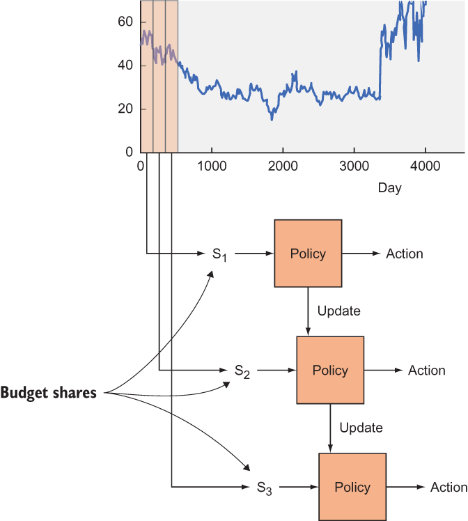
Figure 13.8 A rolling window of a certain size iterates through the stock prices, as shown by the chart segmented into states S1, S2, and S3. The policy suggests an action to take: you may choose to exploit it or randomly explore another action. As you get rewards for performing an action, you can update the policy function over time.

Listing 13.7 Using a given policy to make decisions and returning the performance

def run_simulation(policy, initial_budget, initial_num_stocks, prices, hist):
    budget = initial_budget                                              ❶
    num_stocks = initial_num_stocks                                      ❶
    share_value = 0                                                      ❶
    transitions = list()
    for i in range(len(prices) - hist - 1):
        if i % 1000 == 0:
            print('progress {:.2f}%'.format(float(100*i) / 
            ➥ (len(prices) - hist - 1)))
        current_state = np.asmatrix(np.hstack((prices[i:i+hist], budget, 
        ➥ num_stocks)))                                                 ❷
        current_portfolio = budget + num_stocks * share_value            ❸
        action = policy.select_action(current_state, i)                  ❹
        share_value = float(prices[i + hist])
        if action == 'Buy' and budget >= share_value:                    ❺
            budget -= share_value
            num_stocks += 1
        elif action == 'Sell' and num_stocks > 0:                        ❺
            budget += share_value
            num_stocks -= 1
        else:                                                            ❺
            action = 'Hold'
        new_portfolio = budget + num_stocks * share_value                ❻
        reward = new_portfolio - current_portfolio                       ❼
        next_state = np.asmatrix(np.hstack((prices[i+1:i+hist+1], budget, 
        ➥ num_stocks)))
        transitions.append((current_state, action, reward, next_state))
        policy.update_q(current_state, action, reward, next_state)       ❽
 
    portfolio = budget + num_stocks * share_value                        ❾
    return portfolio

❶ Initializes values that depend on computing the net worth of a portfolio

❷ The state is a hist + 2D vector. You’ll force it to be a NumPy matrix.

❸ Calculates the portfolio value

❹ Selects an action from the current policy

❺ Updates portfolio values based on action

❻ Computes a new portfolio value after taking action

❼ Computes the reward from taking an action at a state

❽ Updates the policy after experiencing a new action

❾ Computes the final portfolio worth

To obtain a more robust measurement of success, run the simulation a couple of times and average the results (listing 13.8). Doing so may take a while (perhaps 5 minutes), but your results will be more reliable.

Listing 13.8 Running multiple simulations to calculate average performance

def run_simulations(policy, budget, num_stocks, prices, hist):
    num_tries = 10                                                         ❶
    final_portfolios = list()                                              ❷
    for i in range(num_tries):
        final_portfolio = run_simulation(policy, budget, num_stocks, prices, 
        ➥ hist)                                                           ❸
        final_portfolios.append(final_portfolio)
        print('Final portfolio: ${}'.format(final_portfolio))
    plt.title('Final Portfolio Value')
    plt.xlabel('Simulation #')
    plt.ylabel('Net worth')
    plt.plot(final_portfolios)
    plt.show()

❶ Decides the number of times to rerun the simulations

❷ Stores the portfolio worth of each run in this array

❸ Runs this simulation

In the main function, append the lines in listing 13.9 to define the decision policy, then run simulations to see how the policy performs.

Listing 13.9 Defining the decision policy

if __name__ == '__main__':
    prices = get_prices('MSFT', '1992-07-22', '2016-07-22')
    plot_prices(prices)
    actions = ['Buy', 'Sell', 'Hold']                           ❶
    hist = 3
    policy = RandomDecisionPolicy(actions)                      ❷
    budget = 100000.0                                           ❸
    num_stocks = 0                                              ❹
    run_simulations(policy, budget, num_stocks, prices, hist)   ❺

❶ Defines the list of actions the agent can take

❷ Initializes a random decision policy

❸ Sets the initial amount of money available to use

❹ Sets the number of stocks already owned

❺ Runs simulations multiple times to compute the expected value of your final net worth

Now that you have a baseline to compare your results, let’s implement a neural network approach to learn the Q-function. The decision policy is often called the Q-learning decision policy. Listing 13.10 introduces a new hyperparameter, epsilon, to keep the solution from getting “stuck” when applying the same action over and over. The lower the value of epsilon, the more often it will randomly explore new actions. The Q-function is defined by the function depicted in figure 13.9.

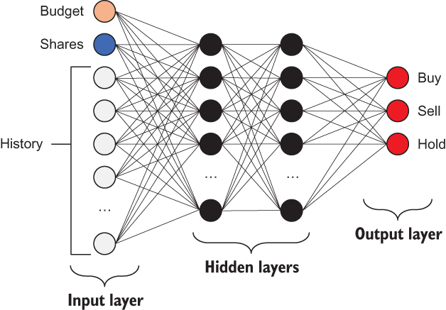
Figure 13.9 input is the state space vector, with three outputs: one for each output’s Q-value

Listing 13.10 Implementing a more intelligent decision policy

class QLearningDecisionPolicy(DecisionPolicy):
    def __init__(self, actions, input_dim):
        self.epsilon = 0.95                                              ❶
        self.gamma = 0.3                                                 ❶
        self.actions = actions
        output_dim = len(actions)
        h1_dim = 20                                                      ❷
        
        self.x = tf.placeholder(tf.float32, [None, input_dim])           ❸
        self.y = tf.placeholder(tf.float32, [output_dim])                ❸
        W1 = tf.Variable(tf.random_normal([input_dim, h1_dim]))          ❹
        b1 = tf.Variable(tf.constant(0.1, shape=[h1_dim]))               ❹
        h1 = tf.nn.relu(tf.matmul(self.x, W1) + b1)                      ❹
        W2 = tf.Variable(tf.random_normal([h1_dim, output_dim]))         ❹
        b2 = tf.Variable(tf.constant(0.1, shape=[output_dim]))           ❹
        self.q = tf.nn.relu(tf.matmul(h1, W2) + b2)                      ❺
        
        loss = tf.square(self.y - self.q)                                ❻
        self.train_op = tf.train.AdagradOptimizer(0.01).minimize(loss)   ❼
        self.sess = tf.Session()                                         ❽
        self.sess.run(tf.global_variables_initializer())                 ❽
    
    def select_action(self, current_state, step):
        threshold = min(self.epsilon, step / 1000.)
        if random.random() < threshold:                                  ❾
               # Exploit best option with probability epsilon
            action_q_vals = self.sess.run(self.q, feed_dict={self.x:  
            ➥ current_state})
            action_idx = np.argmax(action_q_vals)  
            action = self.actions[action_idx]
        else:                                                            ❿
            # Explore random option with probability 1 - epsilon
            action = self.actions[random.randint(0, len(self.actions) - 1)]
        return action
    
    def update_q(self, state, action, reward, next_state):               ⓫
        action_q_vals = self.sess.run(self.q, feed_dict={self.x: state})
        next_action_q_vals = self.sess.run(self.q, feed_dict={self.x: 
        ➥ next_state})
        next_action_idx = np.argmax(next_action_q_vals)
        current_action_idx = self.actions.index(action)
        action_q_vals[0, current_action_idx] = reward + self.gamma * 
        ➥ next_action_q_vals[0, next_action_idx]
        action_q_vals = np.squeeze(np.asarray(action_q_vals))
        self.sess.run(self.train_op, feed_dict={self.x: state, self.y: 
        ➥ action_q_vals})

❶ Sets the hyperparameters from the Q-function

❷ Sets the number of hidden nodes in the neural networks

❸ Defines the input and output tensors

❹ Designs the neural network architecture

❺ Defines the op to compute the utility

❻ Sets the loss as the square error

❼ Uses an optimizer to update model parameters to minimize the loss

❽ Sets up the session and initializes variables

❾ Exploits the best option with probability epsilon

❿ Explores a random option with probability 1 - epsilon

⓫ Updates the Q-function by updating its model parameters

The output from the entire script is shown in figure 13.10. Two key functions are part of the QLearningDecisionPolicy: update_q and select_action, which implement the learned value of actions over time. Five percent of the time, the functions yield a random action. In select_action, every 1,000 or so prices, the function forces a random action and exploration as defined by self.epsilon. In update_q, the agent takes the current state and next desired action as defined by the argmax of q policy value for those states. Because the algorithm is initialized with a Q-function and weights with tf.random_normal, it will take some actions over time for the agent to start to realize the true longer-term reward, but then again, that realization is the point. The agent starts with a random understanding, takes actions, and learns the optimal policy over the simulation.

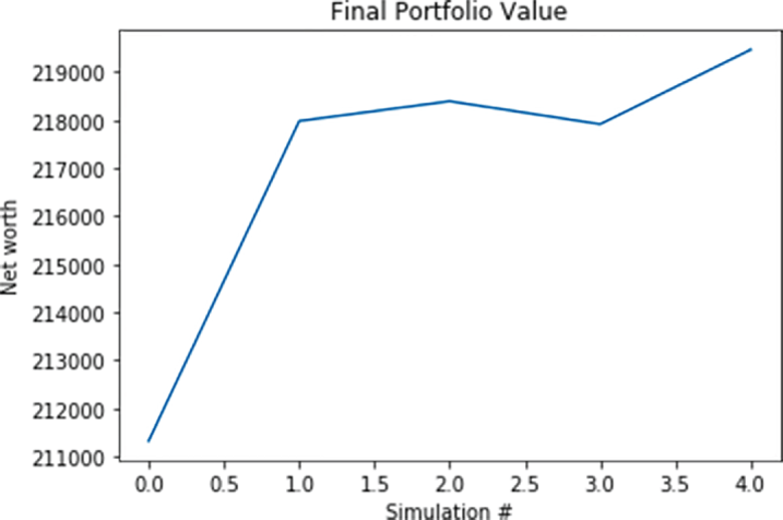
Figure 13.10 The algorithm learns a good policy for trading Microsoft stock.

You can imagine the neural network for the Q-policy function learning to resemble the flow shown in figure 13.11. X is your input, representing the history of three stock prices along with the current balance and number of stocks. The first hidden layer (20, 1) learns a history over time of the reward for particular actions, and the second hidden layer (3, 1) maps those actions to the probability of Buy, Sell, Hold at any time.

Figure 13.11 The neural architecture construction for the Q-policy function with two hidden layers

13.4 Exploring other applications of reinforcement learning

Reinforcement learning is more common than you might expect. It’s too easy to forget that it exists when you’ve learned supervised- and unsupervised-learning methods. But the following examples will open your eyes to successful uses of RL by Google:

• Game playing —In February 2015, Google developed a reinforcement-learning system called Deep RL to learn how to play arcade video games from the Atari 2600 console. Unlike most RL solutions, this algorithm had a high-dimensional input; it perceived the raw frame-by-frame images of the video game. That way, the same algorithm could work with any video game without much reprogramming or reconfiguring.

• More game playing —In January 2016, Google released a paper about an AI agent that was capable of winning the board game Go. The game is known to be unpredictable because of the enormous number of possible configurations (even more than in chess!), but this algorithm, using RL, could beat top human Go players. The latest version, AlphaGo Zero, was released in late 2017 and was able to beat the earlier version consistently—100 games to 0—in only 40 days of training. AlphaGo Zero will be considerably better than its 2017 performance by the time you read this book.

• Robotics and control —In March 2016, Google demonstrated a way for a robot to learn how to grab an object via many examples. Google collected more than 800,000 grasp attempts by using multiple robots and developed a model to grasp arbitrary objects. Impressively, the robots were capable of grasping an object with the help of camera input alone. Learning the simple concept of grasping an object required aggregating the knowledge of many robots, spending many days in brute-force attempts until enough patterns were detected. Clearly, robots have a long way to go to be able to generalize, but this project is an interesting start nonetheless.

Note Now that you’ve applied reinforcement learning to the stock market, it’s time for you to drop out of school or quit your job and start gaming the system—your payoff, dear reader, for making it this far into the book! I’m kidding. The actual stock market is a much more complicated beast, but the techniques in this chapter generalize to many situations.

Summary

• Reinforcement learning is a natural tool for problems that can be framed by states that change due to actions taken by an agent to discover rewards.

• Implementing the reinforcement-learning algorithm requires three primary steps: infer the best action from the current state, perform the action, and learn from the results.

• Q-learning is an approach to solving reinforcement learning whereby you develop an algorithm to approximate the utility function (Q-function). After a good enough approximation is found, you can start inferring the best actions to take from each state.