
In the previous chapters, I have repeatedly demonstrated how ANNs and CNNs can classify a variety of objects including handwritten numbers and clothing articles. In this chapter I will explore how ANNs and CNNs can predict an outcome. I have noticed repeatedly that DL practitioners often conflate classification and prediction. This is understandable because these tasks are closely intertwined. For instance, when presented with an unknown Image, a CNN will attempt to identify it as belonging to one of the classes it has been trained to recognize. This is clearly a classification process. However, if just view this process from a wider perspective, you could say the CNN has been tasked to predict what the Image represents. I choose to take the narrower view and restrict my interpretation of prediction, at least as far as it concerns ANNs and CNNs to the following definition:
Prediction refers to the output of a DL algorithm after it has been trained on a dataset and when new data is applied to forecast the Likelihood of a particular outcome.
The word prediction can also be misleading. In some cases, it does mean that a future outcome is being predicted, such as when you’re using DL to determine the next best action to take in a marketing campaign. In other cases, the prediction has to do with whether or not a transaction that has already occurred was a fraud. In that case, the transaction has already happened and the algorithm is making an educated guess about whether or not it was legitimate. My initial demonstration is very straightforward and the ANN will make a binary choice when presented with a set of facts. The choice is whether or not the applied record is part of a class or is not. This last statement will become quite clear when I next present the demonstration.
Pima Indian Diabetes demonstration
The Pima Indian Diabetes project is another one of the classic problems that DL students always study. It is an excellent case study on how an ANN can make predictions based on an applied record when that ANN has been thoroughly trained on an historical dataset.
Background for the Pima Indian Diabetes study
Diabetes mellitus is a group of metabolic disorders where the blood sugar levels are higher than normal for prolonged periods of time. Diabetes is caused either due to the insufficient production of insulin in the body or due to improper response of the body’s cells to insulin. The former cause of diabetes is also called type 1 DM or insulin-dependent diabetes mellitus, and the latter is known as type 2 DM or non-insulin-dependent DM. Gestational diabetes is a third type of diabetes where women not suffering from DM develop high sugar levels during pregnancy. Diabetes is especially hard on women as it can affect both the mother and their unborn children during pregnancy. Women with diabetes have a higher Likelihood at having a heart attack, miscarriages, or babies born with birth defects
The diabetes data containing information about Pima Indian females, near Phoenix, Arizona, has been under continuous study since 1965 due to the high incidence rate of diabetes in Pima females. The dataset was originally published by the National Institute of Diabetes and Digestive and Kidney Diseases, consisting of diagnostic measurements pertaining to females of age greater than 20. It contains information of 768 females, of which 268 females were diagnosed with diabetes. Information available includes eight variables which are detailed in Table 7-1. The response variable in the dataset is a binary classifier, Outcome, that indicates if the person was diagnosed with diabetes or not.
Table 7-1
Eight factors in the Pima Indian Diabetes Study
Variable name | Data type | Variable description |
|---|---|---|
Pregnancies | integer | Number of times pregnant |
Glucose | integer | Plasma glucose concentration at 2 hours in an oral glucose tolerance test |
BloodPressure | integer | Diastolic blood pressure |
SkinThickness | integer | Triceps skin-fold thickness |
Insulin | integer | 2-hour serum insulin (μU/ml) |
BMI | numeric | Body mass index |
DiabetesPedigreeFunction | numeric | Synthesis of the history of diabetes mellitus in relatives, generic relationship of those relatives to the subject |
Outcome | integer | Occurrence of diabetes |
Preparing the data
The first thing you will need to do is download the dataset. This dataset is available from several web sites. I used the following one:
www.kaggle.com/kumargh/pimaindiansdiabetescsv
This download was in an archive format. After extracting it, I renamed the file diabetes.csv just to keep it short and memorable.
The next thing you should do is inspect the data and see if it appears proper and nothing strange or unusual is visible. I used the Microsoft Excel application to do my initial inspection because this dataset was in the CSV format, which is nicely handled by Excel. Figure 7-1 shows the first 40 of 768 rows from the dataset.
Figure 7-1
First 40 rows from the diabetes.csv dataset
What immediately stood out to me was the inordinate amount of zeros present both in the SkinThickness and Insulin columns. There should not be any zeros in these columns because a living patient can neither have zero skin thickness nor zero insulin levels. This prompted me to do a bit of research, and I determined that the original researchers who built this dataset simply inserted zeros for empty or null readings. This practice is totally unacceptable and may corrupt a dataset to the point where it could easily generate false or misleading results when processed by an ANN. So, what could I do about it?
Further research on my part leads to the following process, which “corrected” for the missing values in a reasonable manner and also illustrated a nice way to visualize the data. I like to give credit to Paul Mooney and his blog “Predict Diabetes from Medical Records” for providing useful insights into solving this issue. Paul used a Python notebook format for his computations. I changed and modified his interactive commands into conventional Python scripts for this discussion.
Please ensure you are in a Python virtual environment prior to beginning this session. You will then need to ensure that the Seaborn, Matplotlib, and Pandas libraries are installed prior to running the script. Enter the following commands to install these libraries if you are unsure they are present:
pip install seaborn
pip install matplotlib
pip install pandas
The following script loads the diabetes.csv dataset and then does a series of data checks, summaries, and histogram plots. I named this script diabetesTest.py, and it is available from the book’ companion web site. I also included some explanatory comments after the script to help clarify what is happening within it.
# Import required libraries
import matplotlib.pyplot as plt
import seaborn as sns
import pandas as pd
# Load the CSV dataset
dataset = pd.read_csv('diabetes.csv')
dataset.head(10)
# Define a histogram plot method
def plotHistogram(values, label, feature, title):
sns.set_style("whitegrid")
plotOne = sns.FacetGrid(values, hue=label, aspect=2)
plotOne.map(sns.distplot, feature, kde=False)
plotOne.set(xlim=(0, values[feature].max()))
plotOne.add_legend()
plotOne.set_axis_labels(feature, 'Proportion')
plotOne.fig.suptitle(title)
plt.show()
# Plot the Insulin histogram
plotHistogram(dataset, 'Outcome', 'Insulin', 'Insulin vs Diagnosis (Blue = Healthy; Orange = Diabetes)')
# Plot the SkinThickness histogram
plotHistogram(dataset, 'Outcome', 'SkinThickness', 'SkinThickness vs Diagnosis (Blue = Healthy; Orange = Diabetes)')
# Summary of the number of 0's present in the dataset by feature
dataset2 = dataset.iloc[:, :-1]
print("Num of Rows, Num of Columns: ", dataset2.shape)
print("
Column Name Num of Null Values
")
print((dataset[:] == 0).sum())
# Percentage summary of the number of 0's in the dataset
print("Num of Rows, Num of Columns: ", dataset2.shape)
print("
Column Name %Null Values
")
print(((dataset2[:] == 0).sum()) / 768 * 100)
# Create a heat map
g = sns.heatmap(dataset.corr(), cmap="BrBG", annot=False)
plt.show()
# Display the feature correlation values
corr1 = dataset.corr()
print(corr1[:])
Explanatory comments:
- dataset = pd.read_csv('diabetes.csv') – Reads the CSV dataset into the script using the Pandas read_csv method.
- dataset.head(10) – Displays the first ten records in the dataset.
- def plotHistogram(values, label, feature, title) – Defines a method which will plot the histogram of the dataset feature provided in the arguments list. This method uses the Seaborn library, which I discussed in Chapter 2. Two histograms are then plotted after this definition, one for Insulin and the other for SkinThickness. Each of those features had a significant amount of 0s present.
- dataset2 = dataset.iloc[:, :-1] – Is the start of the code segment which displayed the actual amount of 0s present for each dataset feature. The only features that should have any 0s are Outcome and Pregnancies.
- print("Num of Rows, Num of Columns: ", dataset2.shape) – Is the start of the code segment which displayed the percentages of 0s present for each dataset feature.
- g = sns.heatmap(dataset.corr(), cmap="BrBG", annot=False) – Generates a heatmap for the dataset’s correlation map. A heatmap is a way of representing the data in a 2D form. Data values are represented as colors in the graph. The goal of the heatmap is to provide a colored visual summary of information.
- corr1 = dataset.corr() – Creates a table of correlation values between the dataset feature variables. This statistic will be of considerable interest after the values in the dataset have been adjusted.
This script should be run in the virtual environment with the diabetes.csv dataset in the same directory as this script. Enter the following command to run the script:
python diabetesTest.py
This script runs immediately and produces a series of results. The final screen results are shown in Figure 7-2.
Figure 7-2
Final results after running the diabetesTest script
The first table in the figure lists the nulls (0s) for each feature. There is clearly an unacceptable amount of 0s in both the SkinThickness and Insulin feature columns. Almost 50% of the Insulin data points are missing, which you can easily see from looking at the next table in the figure. There will be an inadvertent bias introduced into any ANN, which uses this dataset because of these missing values. How it will affect the overall ANN prediction performance is uncertain, but it will be an issue nonetheless.
The last table in the figure shows the correlation values between the feature variables. Usually, I would like to see low values between the variables except for those features which are naturally related such as age and pregnancies. You should also note that this table is a symmetric matrix around the identity diagonal. The identity diagonal (all 1s) results because the correlation value for a variable with itself must always equal to 1. The symmetric matrix results because the correlation function is commutative (order of variables does not matter). The key value I will be looking for is how the current correlation value of 0.436783 between SkinThickness and Insulin changes after the data is modified to get rid of the 0s.
Figure 7-3 is the histogram showing the relationship between insulin levels and the proportion of healthy to sick patients.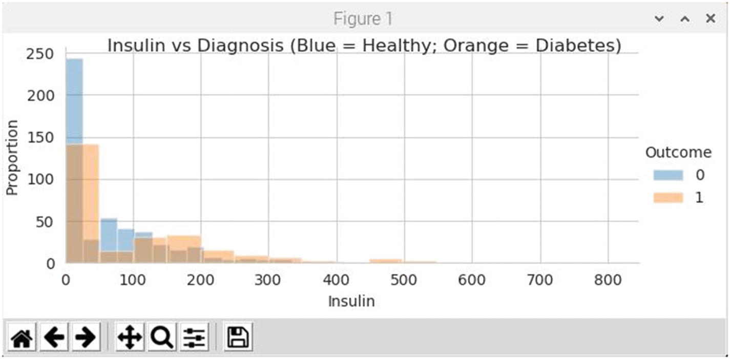
Figure 7-3
Histogram for insulin levels and proportion of healthy to sick patients
There seems to be a strong clustering of unhealthy patients below the 40 level which doesn’t make sense because it is unlikely that any living patient would have such low levels. Additionally, having a strong spike of heathy patients with insulin levels at 20 or below is simply not realistic. They too could not live will such low levels. Clearly the excess 0 problem is skewing the data and causing the ANN to make erroneous predictions.
Figure 7-4 is the histogram showing the relationship between skin thickness measurements and the proportion of healthy to sick patients.
Figure 7-4
Histogram for skin thickness measurements and proportion of healthy to sick patients
In this figure, just like the previous figure, there are abnormal spikes in the skin thickness measurements for both healthy and sick patients near the 0 skin thickness measurement. It is simply not possible to have 0 skin thickness. The excess 0 problem is solely causing this anomaly.
Figure 7-5 shows the heatmap for the correlation matrix between all the dataset feature variables.
Figure 7-5
Correlation heatmap for dataset feature variables
What you should look for in this figure are the white blocks, which indicate correlation values at or above 0.4. Most correlation values for this dataset are relatively low except for
- Glucose and Outcome
- Age and Pregnancies
- Insulin and SkinThickness
The first two in the list make perfect sense. Glucose (sugar levels in the blood) are definitely correlated with diabetes and hence the Outcome. Age and Pregnancies are naturally correlated because women have fewer pregnancies as they age, or if they are young, they haven’t had the time to sustain many pregnancies. The last one in the list is the suspect one, which is an artificially high correlation value due to the excess-zero problem.
It is now time to fix the excess 0’s problem. The question naturally becomes how to do this without causing too much disruption to the dataset? The answer most statisticians would cite is to impute the missing data. Imputing data is a tricky process because it can insert additional bias into the dataset. The process of imputing data can take on several forms depending on the nature of the data. If the data is from a time series, then missing data can easily be replaced by interpolating between the data surrounding the missing values. Unfortunately, the diabetes dataset is not time sensitive, so this option is out.
Another way to impute is to simply eliminate those records with missing data. This is called listwise imputation
. Unfortunately, using listwise imputation would cause nearly 50% of existing dataset records to disappear. This would wreak havoc on the ANN learning process so that option is out. One of the remaining impute options is to use all the existing feature data to determine a value to replace the missing data. There are imputation processes called hot card, cold card, mean, and median value, which use this approach. Without going into the details, I decided to use median value as the option to replace the missing data values.
The following script is a revision of the previous script where I have imputed the dataset to remove all 0s from the feature variables. The dataset has also been split into two dataset, one for training and the other for testing. The script is named revisedDiabetesTest.py and is available from the book’s companion web site. I have also provided some explanatory comments after the listing.
# Import required libraries
import numpy as np
import matplotlib.pyplot as plt
import seaborn as sns
import pandas as pd
from sklearn.model_selection import train_test_split
from sklearn.impute import SimpleImputer
# Load the dataset
data = pd.read_csv('diabetes.csv')
X = data.iloc[:, :-1]
y = data.iloc[:, -1]
# Split the dataset into 80% training and 20% testing sets
X_train, X_test, y_train, y_test = train_test_split(X, y, test_size=0.2, random_state=1)
# Impute the missing values using feature median values
imputer = SimpleImputer(missing_values=0, strategy="median")
X_train2 = imputer.fit_transform(X_train)
X_test2 = imputer.transform(X_test)
# Convert the numpy array into a Dataframe
X_train3 = pd.DataFrame(X_train2)
# Display the first 10 records
print(X_train3.head(10))
def plotHistogram(values, label, feature, title):
sns.set_style("whitegrid")
plotOne = sns.FacetGrid(values, hue=label, aspect=2)
plotOne.map(sns.distplot, feature, kde=False)
plotOne.set(xlim=(0, values[feature].max()))
plotOne.add_legend()
plotOne.set_axis_labels(feature, 'Proportion')
plotOne.fig.suptitle(title)
plt.show()
# Plot the heathy patient histograms for insulin and skin
# thickness
plotHistogram(X_train3,None,4,'Insulin vs Diagnosis')
plotHistogram(X_train3,None,3,'SkinThickness vs Diagnosis')
# Check to see if any 0's remain
data2 = X_train2
print("Num of Rows, Num of Columns: ", data2.shape)
print("
Column Name Num of Null Values
")
print((data2[:] == 0).sum())
print("Num of Rows, Num of Columns: ", data2.shape)
print("
Column Name %Null Values
")
print(((data2[:] == 0).sum()) / 614 * 100)
# Display the correlation matrix
corr1 = X_train3.corr()
print(corr1)
Explanatory comments:
- X_train, X_test, y_train, y_test = train_test_split(X, y, test_size=0.2, random_state=1) – Splits the input dataset into two, one 80% of the input for training purposes and the other 20% for testing purposes
- X_train3 = pd.DataFrame(X_train2) – Converts the training dataset from a numpy array into a Pandas DataFrame so it is compatible with the Pandas cross-correlation function
Again, this script should be run in the virtual environment with the diabetes.csv dataset in the same directory as this script. Enter the following command to run the script:
python revisedDiabetesTest.py
This script runs immediately and produces a series of results. The final screen results are shown in Figure 7-6.
Figure 7-6
Final results after running the revisedDiabetesTest script
You can immediately see that all 0 values in the first ten training set records have been replaced with other values. This is true for all of the feature variables, but not the Outcome column, which is required for supervised learning.
The 0 summary code displays now that there are no 0s remaining in the dataset.
Figure 7-7 is the revised histogram showing the insulin distribution for healthy patients. There is no longer any insulin values at or near 0. The distribution peak is centered around 130, which seems reasonable to me, but again, I am not an MD.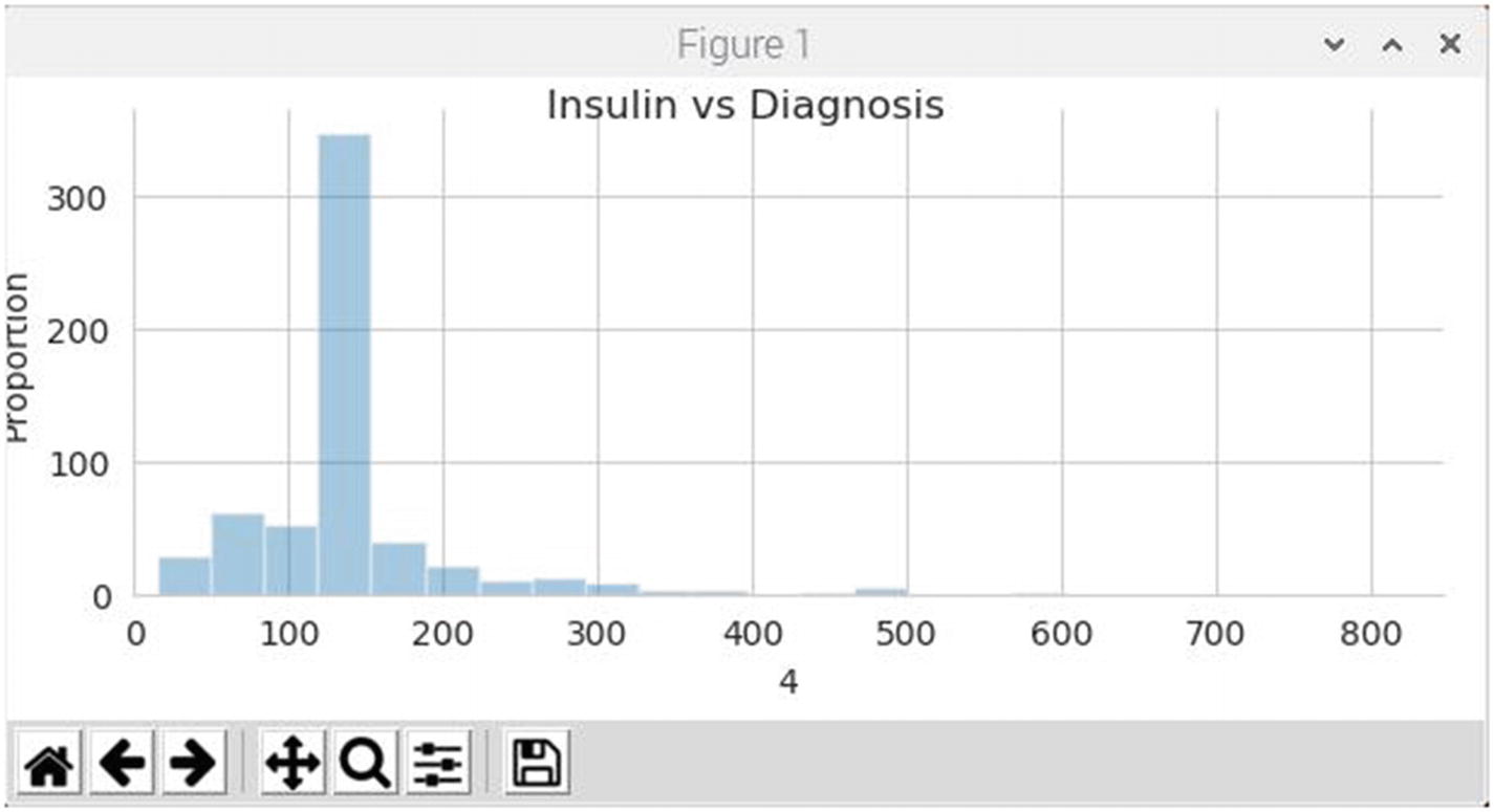
Figure 7-7
Insulin histogram for healthy patients
Figure 7-8 is the revised histogram showing the skin thickness distribution for healthy patients. As was the case for the insulin plot, this plot shows no values whatsoever below 8. The peak appears to center on a value of 29, which I presume is a reasonable number.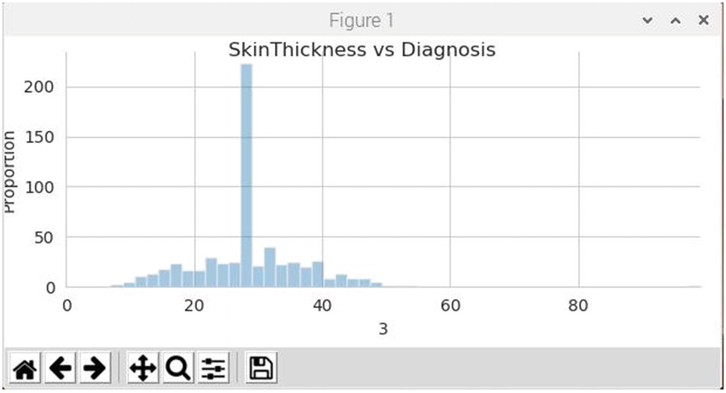
Figure 7-8
Skin thickness histogram for healthy patients
The correlation matrix shown at the bottom of Figure 7-6 now shows a significantly decreased correlation value between insulin and skin thickness. Before the 0s were removed, the correlation value between these two features was 0.436783. It is now 0.168746, which is about a 61% reduction. The 0 removal definitely improved the data quality, at least with these two features.
It is time to discuss the Keras ANN model
now that the dataset has been “cleaned up” into a better state. The model to be built will be a relatively simple three-layer, sequential one. The input layer will have eight inputs corresponding to the eight dataset feature variables. Fully connected layers will be used in the model using the Keras dense class. The ReLU activation function will be used for the first two layers because it has been found to be a best performance function. The third layer, which is the output, will use the sigmoid function for activation because the output must be between 0 and 1. Recall this is a prediction model and the output is binary with only either a 0 or 1 value. In summary the model assumptions are
- Expects rows of data with eight variables (the input_dim=8 argument).
- The first hidden layer has 12 nodes and uses the ReLU activation function.
- The second hidden layer has eight nodes and uses the ReLU activation function.
- The output layer has one node and uses the sigmoid activation function.
Note that the first hidden layer is actually performing two functions. It is acting as an input layer in accepting eight variables, and it is also acting as a hidden layer with 12 nodes with associated ReLU activation functions.
The following script is named kerasDiabetesTest.py, and it is available from the book’s companion web site. Explanatory comments follow the listing.
# Import required libraries
import numpy as np
import pandas as pd
from sklearn.model_selection import train_test_split
from sklearn.impute import SimpleImputer
from keras.models import Sequential
from keras.layers import Dense
# Load the dataset
data = pd.read_csv('diabetes.csv')
X = data.iloc[:, :-1]
y = data.iloc[:, -1]
# Split the dataset into 80% training and 20% testing sets
X_train, X_test, y_train, y_test = train_test_split(X, y, test_size=0.2, random_state=1)
# Impute the missing values using feature median values
imputer = SimpleImputer(missing_values=0,strategy='median')
X_train2 = imputer.fit_transform(X_train)
X_test2 = imputer.transform(X_test)
# Convert the numpy array into a Dataframe
X_train3 = pd.DataFrame(X_train2)
# Define the Keras model
model = Sequential()
model.add(Dense(12, input_dim=8, activation="relu"))
model.add(Dense(8, activation="relu"))
model.add(Dense(1, activation="sigmoid"))
# Compile the keras model
model.compile(loss='binary_crossentropy', optimizer="adam", metrics=['accuracy'])
# fit the keras model on the dataset
model.fit(X_train2, y_train, epochs=150, batch_size=10)
# Evaluate the keras model
_, accuracy = model.evaluate(X_test2, y_test)
print('Accuracy: %.2f' % (accuracy*100))
The first part of the script is the same as the first part of the revisedDiabetesTest.py script with the exception of some added and deleted imports. The model definition is in line in lieu of a separate definition as was the case for the CNN scripts. This was done because it is a very simple and concise model. The compile process is almost the same as it was for the CNN models, except for the loss function, which is binary_crossentropy instead of categorical_crossentropy
, which is required for multiple classes. This model will train and test very quickly, which allows for many epochs to be run in an effort to improve the accuracy. In this case, there are 150 epochs set. The overall accuracy is done using the Keras evaluate method as it was done for the CNN models.
This script should be run in the virtual environment with the diabetes.csv dataset in the same directory as this script. Enter the following command to run the script:
python kerasDiabetesTest.py
This script runs immediately and produces a series of results. The final screen results are shown in Figure 7-9.
Figure 7-9
Final results after running the kerasDiabetesTest script
This figure is a composite showing the beginning and ending epoch results. The final, overall accuracy score was 70.78%. This would normally be considered an OK, but not great score. However, I did some research on others who have run this project with similar models and found that this result was in line with the majority of other results. It appears that the Pima Indian Diabetes Study predictions are approximately successful (or accurate) around 70% of the time. I believe that this level of accuracy would not be an acceptable level if used in actual clinical trials, but is perfectly acceptable in this learning and experimentation environment.
Using the scikit-learn library with Keras
The Python scikit-learn library uses the scipy stack for efficient numerical computations. It is a fully featured library for general ML library that provides many utilities which are useful in the developing models. These utilities
include
- Model evaluation using resampling methods such as k-fold cross-validation
- Efficient evaluation of model hyper-parameters
The Keras library is a convenient wrapper for DL models used for classification or regression estimations with the scikit-learn library.
The following demonstration uses the KerasClassifier wrapper for a classification neural network created in Keras and is used with the scikit-learn library. I will also be using the same modified Pima Indian Diabetes dataset that is used in the last demonstration.
This demonstration script is very similar to the previous one in that it uses the same Keras ANN model. The significant difference is that in this script the model is used by the KerasClassifier instead of having the modified dataset directly applied to the model via the Keras fit function. I will explain how the KerasClassifier works after the script listing because it is important for you to see how it is invoked.
The following script is named kerasScikitDiabetesTest.py to indicate that it now uses the scikit-learn classifier in lieu of the normal Keras fit function. It is available from the book’s companion web site.
# Load required libraries
from keras.models import Sequential
from keras.layers import Dense
from keras.wrappers.scikit_learn import KerasClassifier
from sklearn.model_selection import StratifiedKFold
from sklearn.model_selection import cross_val_score
from sklearn.model_selection import train_test_split
from sklearn.impute import SimpleImputer
import pandas as pd
# Function to create model, required for the KerasClassifier
def create_model():
# create model
model = Sequential()
model.add(Dense(12, input_dim=8, activation="relu"))
model.add(Dense(8, activation="relu"))
model.add(Dense(1, activation="sigmoid"))
model.compile(loss='binary_crossentropy', optimizer="adam", metrics=['accuracy'])
return model
# fix random seed for reproducibility
seed = 42
# Load the dataset
data = pd.read_csv('diabetes.csv')
X = data.iloc[:, :-1]
y = data.iloc[:, -1]
# Split the dataset into 80% training and 20% testing sets
X_train, X_test, y_train, y_test = train_test_split(X, y, test_size=0.2, random_state=1)
# Impute the missing values using feature median values
imputer = SimpleImputer(missing_values=0,strategy='median')
X_train2 = imputer.fit_transform(X_train)
X_test2 = imputer.transform(X_test)
# Convert the numpy array into a Dataframe
X_train3 = pd.DataFrame(X_train2)
# create model
model = KerasClassifier(build_fn=create_model, epochs=150, batch_size=10, verbose=0)
# evaluate using 10-fold cross validation
kfold = StratifiedKFold(n_splits=10, shuffle=True, random_state=seed)
# Evaluate using cross_val_score function
results = cross_val_score(model, X_train2, y_train, cv=kfold)
print(results.mean())
This script should be run in the virtual environment with the diabetes.csv dataset in the same directory as this script. Enter the following command to run the script:
python kerasScikitDiabetesTest.py
This script runs immediately and produces a single result. The final screen result is shown in Figure 7-10.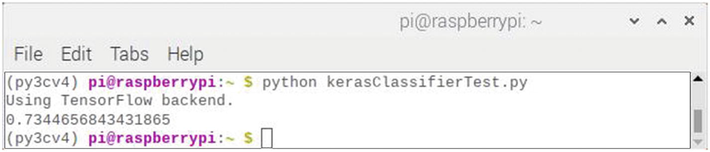
Figure 7-10
Final result after running the kerasScikitDiabetesTest script
The accuracy value displayed in the figure is 73.45%. This value was based on only using the training dataset, which is 80% of the original dataset. Consequently, I reran the script with the split changed to 99% for the training set, which meant it was almost the size of the unsplit dataset. The result was an accuracy was 73.40%, which is a statistically insignificant difference from the first run.
The KerasClassifier and KerasRegressor classes in Keras take an argument named build_fn which is the model’s function name. In the preceding script, a method named create_model()
that creates a MLP for this case. This function is passed to the KerasClassifier class by the build_fn argument. There are additional arguments of nb_epoch=150 and batch_size=10 that are automatically used by the fit() function, which is called internally by the KerasClassifier class.
In this example, the scikit-learn StratifiedKFold function
is then used to perform a tenfold stratified cross-validation. This is a resampling technique that provides a robust estimate of the accuracy for the defined model with the applied dataset.
The scikit-learn function cross_val_score is used to evaluate the model using a cross-validation scheme and display the results.
Grid search with Keras and scikit-learn
In this follow-on demonstration, a grid search is used to evaluate different configurations for the ANN model. The configuration that produces the best estimated performance is reported.
The create_model() function
is defined with two arguments, optimizer and Init, both of which have default values. Varying these argument values allows for the evaluation of the effect of using different optimization algorithms and weight initialization schemes on the network model.
After model creation, there is a definition of parameter arrays used in the grid search. The search is intended to test
- Optimizers for searching different weight values
- Initializers for preparing the network weights using different schemes
- Epochs for training the model for a different number of exposures to the training dataset
- Batches for varying the number of samples before a weight update
The preceding options are stored in a dictionary and then passed to the configuration of the GridSearchCV scikit-learn class. This class evaluates a version of the ANN model for each combination of parameters (2 x 3 x 3 x 3 for the combinations of optimizers, initializations, epochs, and batches). Each combination is then evaluated using the default threefold stratified cross-validation.
There are a lot of models, and it all takes a considerable amount of computation time as you will find out if you replicate this demonstration using a RasPi. The estimation duration for this RasPi setup is about 2 hours, which is reasonable considering the relatively small network and the small dataset (less than 800 records instances and 9 features and attributes).
After the script has finished, the performance and combination of configurations for the best model are displayed, followed by the performance for all of the combinations of parameters.
The following script is named kerasScikitGridSearchDiabetesTest.py to indicate that it uses the scikit-learn grid search algorithm to help determine the optimal configuration for the ANN model. This script is available from the book’s companion web site:
# Import required libraries
import numpy as np
import pandas as pd
from keras.models import Sequential
from keras.layers import Dense
from sklearn.model_selection import train_test_split
from sklearn.impute import SimpleImputer
from keras.wrappers.scikit_learn import KerasClassifier
from sklearn.model_selection import GridSearchCV
from sklearn.model_selection import cross_val_score
# Function to create model, required for KerasClassifier
def create_model(optimizer='rmsprop', init="glorot_uniform"):
# create model
model = Sequential()
model.add(Dense(12, input_dim=8, kernel_initializer=init, activation="relu"))
model.add(Dense(8, kernel_initializer=init, activation="relu"))
model.add(Dense(1, kernel_initializer=init, activation="sigmoid"))
# Compile model
model.compile(loss='binary_crossentropy', optimizer=optimizer, metrics=['accuracy'])
return model
# Random seed for reproducibility
seed = 42
np.random.seed(seed)
# Load the dataset
data = pd.read_csv('diabetes.csv')
X = data.iloc[:, :-1]
y = data.iloc[:, -1]
# Split the dataset into 80% training and 20% testing sets
X_train, X_test, y_train, y_test = train_test_split(X, y, test_size=0.2, random_state=1)
# Impute the missing values using feature median values
imputer = SimpleImputer(missing_values=0,strategy='median')
X_train2 = imputer.fit_transform(X_train)
X_test2 = imputer.transform(X_test)
# Convert the numpy array into a Dataframe
X_train3 = pd.DataFrame(X_train2)
# Create model
model = KerasClassifier(build_fn=create_model, verbose=0)
# Grid search epochs, batch size and optimizer
optimizers = ['rmsprop', 'adam']
init = ['glorot_uniform', 'normal', 'uniform']
epochs = [50, 100, 150]
batches = [5, 10, 20]
param_grid = dict(optimizer=optimizers, epochs=epochs, batch_size=batches, init=init)
grid = GridSearchCV(estimator=model, param_grid=param_grid)
grid_result = grid.fit(X_train2, y_train)
# Summarize results
print("Best: %f using %s" % (grid_result.best_score_, grid_result.best_params_))
means = grid_result.cv_results_['mean_test_score']
stds = grid_result.cv_results_['std_test_score']
params = grid_result.cv_results_['params']
for mean, stdev, param in zip(means, stds, params):
print("%f (%f) with: %r" % (mean, stdev, param))
This script should be run in the virtual environment with the diabetes.csv dataset in the same directory as this script. Enter the following command to run the script:
python kerasScikitGridSearchDiabetesTest.py
This script takes about 2 hours to complete because of the many sets of epochs being run. The final screen results are shown in Figure 7-11, which is a composite that I made showing the beginning and ending set of epoch interim results.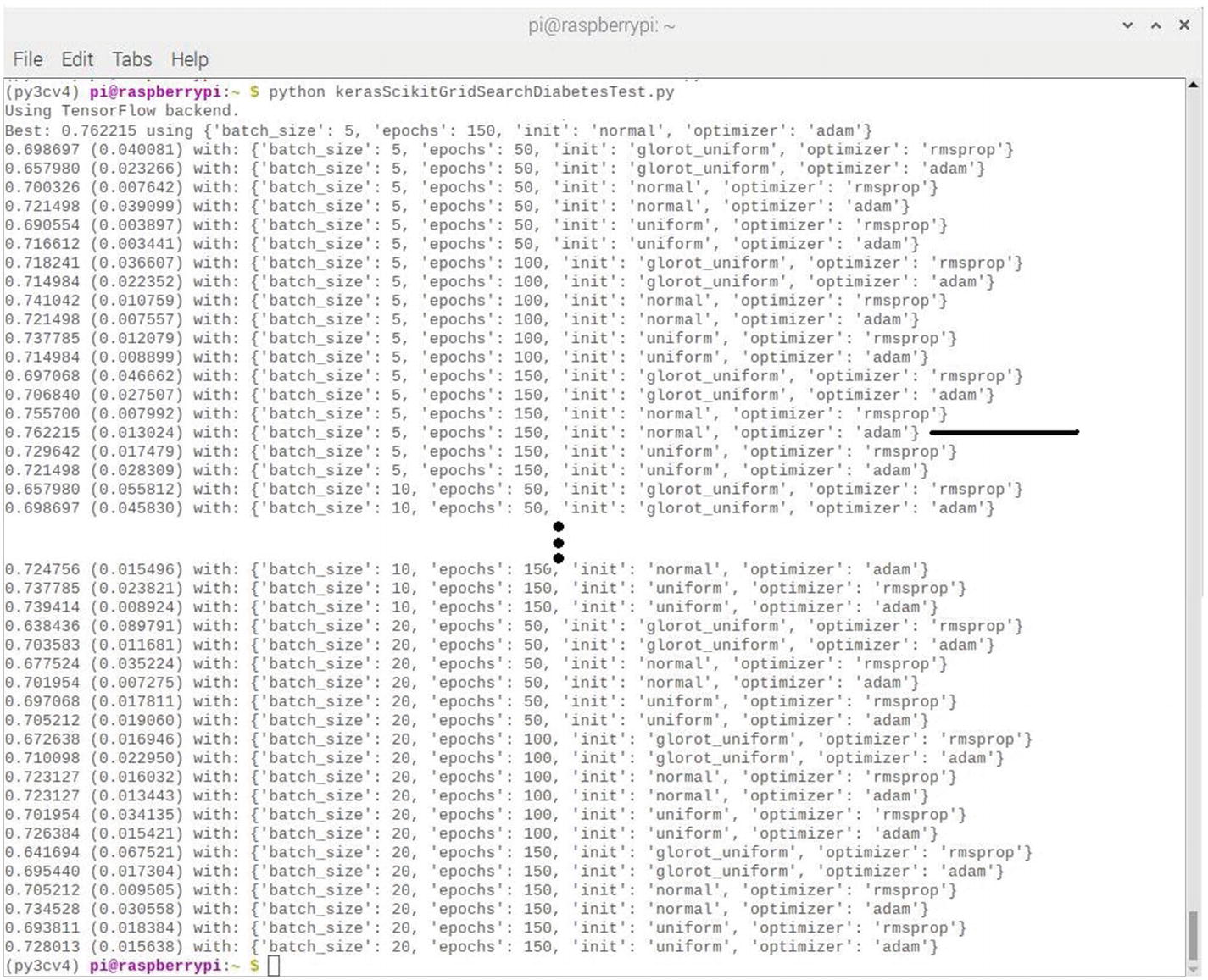
Figure 7-11
Final results after running the kerasScikitGridSearchDiabetesTest script
The highest accuracy achieved for all the sets of epochs run was 76.22%. Note that I drew line pointing to the optimal set in the figure. This set was configured for 150 epochs, a batch size of 5, a normal distribution, and the Adam optimizer.
Housing price regression predictor demonstration
Modern online property companies offer valuations of houses using ML techniques. This demonstration will predict the prices of houses in the metropolitan area of Boston, MA (USA), using an ANN and a scikit-learn multiple linear regression (MLR) function. The dataset used in this demonstration is rather dated (1978), but it is still adequate for the purposes of this project.
The dataset consisted of 13 variables and 507 records. The dataset feature variables
are detailed in Table 7-2.
Table 7-2
Boston housing dataset feature variables
Columns | Description |
|---|---|
CRIM | Per capita crime rate by town |
ZN | Proportion of residential land zoned for lots over 25,000 sq. ft. |
INDUS | Proportion of non-retail business acres per town |
CHAS | Charles River dummy variable (= 1 if tract bounds river; 0 otherwise) |
NOX | Nitric oxide concentration (parts per 10 million) |
RM | Average number of rooms per dwelling |
AGE | Proportion of owner-occupied units built prior to 1940 |
DIS | Weighted distances to five Boston employment centers |
RAD | Index of accessibility to radial highways |
TAX | Full-value property tax rate per $10,000 |
PTRATIO | Pupil-teacher ratio by town |
LSTAT | Percentage of lower status of the population |
MEDV | Median value of owner-occupied homes in $1000s |
The price of the house indicated by the variable MEDV is the target variable
, and the remaining features are the feature variables on which the value of a house will be predicted.
Preprocessing the data
It is always good practice to become familiar with the dataset to be used in a project. The obvious first step is to download the dataset. Fortunately, this dataset is readily available using the scikit-learn repository. The following statements will download the dataset into a script:
from sklearn.datasets import load_boston
boston_dataset = load_boston()
I next created a small script to investigate the dataset characteristics including the keys and first few records. I named this script inspectBoston.py, and it is available from the book’s companion web site.
# Load the required libraries
import pandas as pd
from sklearn.datasets import load_boston
# Load the Boston housing dataset
boston_dataset = load_boston()
# Display the dataset keys
print(boston_dataset.keys())
# Display the first five records
boston = pd.DataFrame(boston_dataset.data, columns=boston_dataset.feature_names)
print(boston.head())
# Display the extensive dataset description key
print(boston_dataset.DESCR)
Run this script by using this command:
python inspectBoston.py
Figure 7-12 shows the result of running this script session.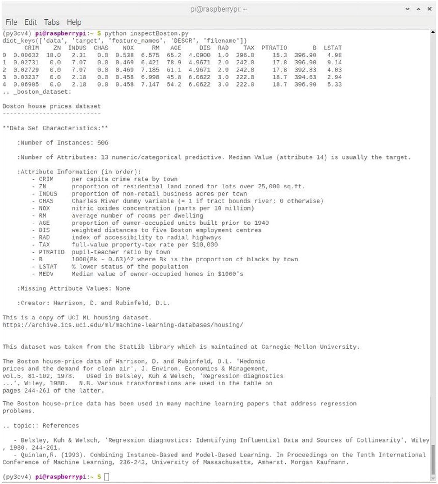
Figure 7-12
Results after running the inspectBoston script
The DESCR portion of the dataset keys is extensive and provides an unusual and comprehensive historical review for this useful dataset. I wish other ML datasets would include such informative data.
Reviewing the initial five records reveals that the target variable MEDV is missing from the DataFrame. This is easily remedied by adding this line of code:
boston['MEDV'] = boston_dataset.target
One quick dataset check that is easy to implement and quite useful is to check for any missing or 0 values in the dataset. This can be done using the isnull() method
along with a summing operation. The statement to do this is
boston.isnull().sum()
I incorporated this null check along with the MEDV correction into a revised inspectBoston script. This revised script, which is now named inspectBostonRev.py, does not display the extensive description as shown in the original script. This script is available from the book’s companion web site:
# Load the required libraries
import pandas as pd
from sklearn.datasets import load_boston
# Load the Boston housing dataset
boston_dataset = load_boston()
# Display the dataset keys
print(boston_dataset.keys())
# Create the boston Dataframe
boston = pd.DataFrame(boston_dataset.data, columns=boston_dataset.feature_names)
# Add the target variable to the Dataframe
boston['MEDV'] = boston_dataset.target
# Display the first five records
print(boston.head())
# Check for null values in the dataset
print(boston.isnull().sum())
Run this script by using this command:
python inspectBostonRev.py
Figure 7-13 shows the result of running this script session.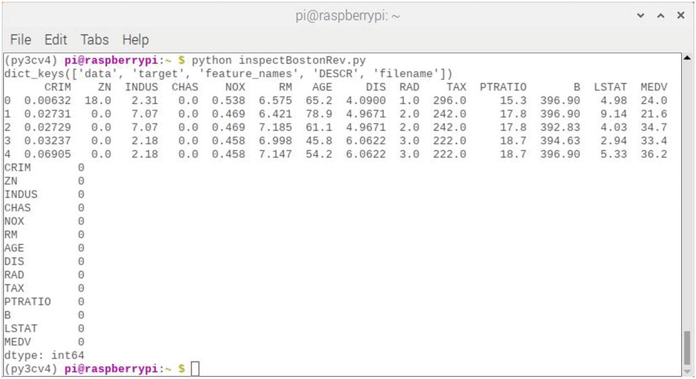
Figure 7-13
Results after running the inspectBoston script
The results display shows that the MEDV target variable has been successfully added to the DataFrame and that there are no null or 0 values present in the dataset. Based on all of the preceding checks, I would say that this dataset was ready to be applied to a model.
The baseline model
A MLP Keras model will first be created and then used with a scikit-learn wrapper regression function to evaluate the Boston housing dataset. This action is almost identical to what happened in the first chapter demonstration where the scikit-learn wrapper function was a classifier instead of a regression package. This method of using Keras models with scikit-learn wrapper functions
is quite powerful because it allows for the use of easy-to-build Keras models with the impressive evaluation capabilities built in with the scikit-learn library.
The baseline model is a simple structure with a single fully connected hidden layer with the same number of nodes as the input feature variables (13). The network also uses the efficient ReLU activation functions. However, no activation function is used on the output layer because this network is designed to predict numerical values and does not need any transformations applied.
The Adam optimizer is used and a mean squared error (MSE) loss function is the target function to be optimized. The MSE will also be the same metric used to evaluate the network performance. This is a desirable metric because it can be directly understood in the context of the problem, which is a house price in thousands of dollars squared.
The Keras wrapper object used with the scikit-learn library is named KerasRegressor. This is instantiated using the same argument types as used with the KerasClassifier object. A reference to the model is required along with several parameters (number of epochs and batch size) that are eventually passed to the fit() function, which does the training.
A random number is also used in the script to help generate consist and reproducible results when the script is repeatedly run.
The model is eventually evaluated using a tenfold cross-validation process as I have previously discussed in this and previous chapters. The final metrics are the MSE including the average and standard deviation across all tenfolds for the cross-validation evaluation.
The dataset must be normalized prior to applying it to the model and evaluation framework. This is because it contains values of widely varying magnitude, which you should realize by now is not a good thing for an ANN to attempt to handle. A normalized dataset is also commonly referred to as a standardized dataset. In this case the scikit-learn StandardScaler function is used to normalize (standardize) the data during the model evaluation within each fold of the cross-validation process.
The following script incorporates all the items discussed earlier. It is named kerasRegressionTest.py and is available from the book’s companion web site.
# Import required libraries
import pandas as pd
from keras.models import Sequential
from keras.layers import Dense
from keras.wrappers.scikit_learn import KerasRegressor
from sklearn.model_selection import cross_val_score
from sklearn.model_selection import KFold
from sklearn.preprocessing import StandardScaler
from sklearn.pipeline import Pipeline
from sklearn.datasets import load_boston
# Load the Boston housing dataset
boston_dataset = load_boston()
# Create the boston Dataframe
dataframe = pd.DataFrame(boston_dataset.data, columns=boston_dataset.feature_names)
# Add the target variable to the dataframe
dataframe['MEDV'] = boston_dataset.target
# Setup the boston dataframe
boston = dataframe.values
# Split into input (X) and output (y) variables
X = boston[:,0:13]
y = boston[:,13]
# Define the base model
def baseline_model():
# Create model
model = Sequential()
model.add(Dense(13, input_dim=13, kernel_initializer='normal', activation="relu"))
model.add(Dense(1, kernel_initializer="normal"))
# Compile model
model.compile(loss='mean_squared_error', optimizer="adam")
return model
# Random seed for reproducibility
seed = 42
# Create a regression object
estimator = KerasRegressor(build_fn=baseline_model, epochs=100, batch_size=5, verbose=0)
# Evaluate model with standardized dataset
estimators = []
estimators.append(('standardize', StandardScaler()))
estimators.append(('mlp', KerasRegressor(build_fn=baseline_model, epochs=50, batch_size=5, verbose=0)))
pipeline = Pipeline(estimators)
kfold = KFold(n_splits=10, random_state=seed)
results = cross_val_score(pipeline, X, y, cv=kfold)
print("Standardized: %.2f (%.2f) MSE" % (results.mean(), results.std()))
Run this script by using this command:
python kerasRegressionTest.py
Figure 7-14 shows the result of running this script session.
Figure 7-14
Results after running the kerasRegressionTest script
The resulting MSE was 28.65, which is not a bad result. For those readers that have some difficulty in working with a statistical measure such as MSE, I will offer a somewhat naive interpretation but perhaps a bit intuitive. I did the following brief set of calculations:
- Mean of all the MEDV values = 22.49 (That’s 1978 house prices in the Boston area)
- Square root of MSE = 5.35
- Ratio of square root of MSE to mean = 0.238
- 1 - above value = 0.762 or “accuracy” = 76.2%
Now, before statisticians start yelling at me, I only present the preceding calculations to provide a somewhat meaningful interpretation of the MSE metric. Clearly an MSE approaching 0 is ideal, but as you can see from this approach, the model is reasonably accurate. In fact, I did some additional research regarding the results of other folks who have used this same dataset and similar networks. I found that the reported accuracies were in the range of 75 to 80%, so this demonstration was right where it should have been.
Improved baseline model
One of the great features of the preceding script is that changes can be made in the baseline model not affecting any other parts of the script. That inherent feature is another subtle example of high cohesion, loose coupling
that I mentioned earlier. Another layer will be added to the model in an effort to improve its performance. This “deeper” model “may” allow the model to extract and combine higher ordered features embedded in the data, which in turn will allow for better predictive results. The code for this model is
# define the model
def larger_model():
# create model
model = Sequential()
model.add(Dense(13, input_dim=13, kernel_initializer="normal", activation="relu"))
model.add(Dense(6, kernel_initializer="normal", activation="relu"))
model.add(Dense(1, kernel_initializer="normal"))
# Compile model
model.compile(loss='mean_squared_error', optimizer="adam")
return model
The modified script was renamed to kerasDeeperRegressionTest.py and is listed in the following. It is available from the book’s companion web site.
# Import required libraries
import pandas as pd
from keras.models import Sequential
from keras.layers import Dense
from keras.wrappers.scikit_learn import KerasRegressor
from sklearn.model_selection import cross_val_score
from sklearn.model_selection import KFold
from sklearn.preprocessing import StandardScaler
from sklearn.pipeline import Pipeline
from sklearn.datasets import load_boston
# Load the Boston housing dataset
boston_dataset = load_boston()
# Create the boston Dataframe
dataframe = pd.DataFrame(boston_dataset.data, columns=boston_dataset.feature_names)
# Add the target variable to the dataframe
dataframe['MEDV'] = boston_dataset.target
# Setup the boston dataframe
boston = dataframe.values
# Split into input (X) and output (y) variables
X = boston[:,0:13]
y = boston[:,13]
# Define the model
def larger_model():
# create model
model = Sequential()
model.add(Dense(13, input_dim=13, kernel_initializer="normal", activation="relu"))
model.add(Dense(6, kernel_initializer="normal", activation="relu"))
model.add(Dense(1, kernel_initializer="normal"))
# Compile model
model.compile(loss='mean_squared_error', optimizer="adam")
return model
# Random seed for reproducibility
seed = 42
# Create a regression object
estimator = KerasRegressor(build_fn=larger_model, epochs=100, batch_size=5, verbose=0)
# Evaluate model with standardized dataset
estimators = []
estimators.append(('standardize', StandardScaler()))
estimators.append(('mlp', KerasRegressor(build_fn=larger_model, epochs=50, batch_size=5, verbose=0)))
pipeline = Pipeline(estimators)
kfold = KFold(n_splits=10, random_state=seed)
results = cross_val_score(pipeline, X, y, cv=kfold)
print("Standardized: %.2f (%.2f) MSE" % (results.mean(), results.std()))
Run this script by using this command:
python kerasDeeperRegressionTest.py
Figure 7-15 shows the result of running this script.
Figure 7-15
Results after running the kerasDeeperRegressionTest script
The result from using a deeper model is an MSE equals to 24.19, which is moderately less than the previous result of 28.65. This shows that the new model is better with predictions than the shallower model. I also repeated my naive calculations and came up with an accuracy of 78.13%. This is almost two points higher than the previous script results. The deeper model is definitely a better performer.
Another improved baseline model
Going deeper is not the only way to improve a model. Going wider can also improve a model by increasing the number of nodes in the hidden layer and hopefully increasing the network’s ability to extract latent features. The code for this model is
# Define the wider model
def wider_model():
# create model
model = Sequential()
model.add(Dense(20, input_dim=13, kernel_initializer="normal", activation="relu"))
model.add(Dense(1, kernel_initializer="normal"))
# Compile model
model.compile(loss='mean_squared_error', optimizer="adam")
return model
The modified script was renamed to kerasWiderRegressionTest.py and is listed in the following. It is available from the book’s companion web site.
# Import required libraries
import pandas as pd
from keras.models import Sequential
from keras.layers import Dense
from keras.wrappers.scikit_learn import KerasRegressor
from sklearn.model_selection import cross_val_score
from sklearn.model_selection import KFold
from sklearn.preprocessing import StandardScaler
from sklearn.pipeline import Pipeline
from sklearn.datasets import load_boston
# Load the Boston housing dataset
boston_dataset = load_boston()
# Create the boston Dataframe
dataframe = pd.DataFrame(boston_dataset.data, columns=boston_dataset.feature_names)
# Add the target variable to the dataframe
dataframe['MEDV'] = boston_dataset.target
# Setup the boston dataframe
boston = dataframe.values
# Split into input (X) and output (y) variables
X = boston[:,0:13]
y = boston[:,13]
# Define the wider model
def wider_model():
# create model
model = Sequential()
model.add(Dense(20, input_dim=13, kernel_initializer="normal", activation="relu"))
model.add(Dense(1, kernel_initializer="normal"))
# Compile model
model.compile(loss='mean_squared_error', optimizer="adam")
return model
# Random seed for reproducibility
seed = 42
# Create a regression object
estimator = KerasRegressor(build_fn=wider_model, epochs=100, batch_size=5, verbose=0)
# Evaluate model with standardized dataset
estimators = []
estimators.append(('standardize', StandardScaler()))
estimators.append(('mlp', KerasRegressor(build_fn=wider_model, epochs=50, batch_size=5, verbose=0)))
pipeline = Pipeline(estimators)
kfold = KFold(n_splits=10, random_state=seed)
results = cross_val_score(pipeline, X, y, cv=kfold)
print("Wider: %.2f (%.2f) MSE" % (results.mean(), results.std()))
Run this script by using this command:
python kerasWiderRegressionTest.py
Figure 7-16 shows the result of running this script.
Figure 7-16
Results after running the kerasWiderRegressionTest script
The result from using a wider model is an MSE equals to 26.35, which is a disappointing result because it is moderately higher than the deeper model result of 24.19. This wider result is still less than the original, unmodified version 28.65. The naive accuracy calculation is 77.17%, which is about halfway between the original and deeper model accuracies.
I believe that experimenting with different node numbers will likely change the outcome to the better. The 20 node value used in this demonstration was just a reasoned guess. You can easily double that and see what happens; however, be careful of either over- or underfitting the model.
One more suggestion I have for curious readers is to try a model that incorporates both a deeper and wider architecture. That very well may be the sweet spot for this project.
Predictions using CNNs
Making a prediction using a CNN at first glance (pardon the pun) might seem like a strange task. CNNs are predicated on using Images as input data sources, and the question that naturally arises is what is a “predicted” Image? The answer lies in the intended use of the Images. CNNs are neural networks just like their ANN counterparts. They are only designed to process numerical arrays and matrices, nothing more. How users interpret CNN outputs are entirely up to the users.
In recent years, CNNs have been used in cellular microscopy applications for cancer and other diseases. The prediction in such case is whether or not a patient has a certain diagnosis based on the analysis of microscopic cell Images. This type of analysis is also widely used for radioscopic (x-ray) examinations, where CNNs have been applied to large-scale Images in an effort to assist with patient diagnosis. Medical predictions have enormous consequences, and CNN analysis is only one tool of many that doctors use to assist in their diagnostic efforts. The subject of CNN medical analysis is quite complicated, and I decided to devote the entire next chapter to it.
Another area where CNN predictions are commonly used is with time series analysis, and this one is fortunately not nearly as complicated as the medical diagnosis one. I have included a series of relatively simple demonstrations to illustrate how to use a CNN with a time series. However, I will first answer the obvious question, what is a time series? A time series is just a series of data point indexed in time order. Most commonly, a time series is a numerical sequence sampled at successive equally spaced data points in time. It is only a sequence of discrete, time-related data points. Examples of time series are ocean tide heights, sunspot activity, and the daily closing value of the Dow Jones Industrial Average. The common attribute shared by all-time series is that they are all historical. That is where the CNN comes in. A CNN uses the historical record to predict the next data point. In reality, this is not a big problem if the time series is logical and well ordered. If I presented you with the following time series
- 5, 10, 15, 20, 25, 30, 35, 40, 45, 50, 55, ?
and asked you to predict the next number in the series, I don’t think anyone of my bright readers would have a problem doing that. But, if I presented you with the following sequence
- 86.6, 50, 0, –50, –86.6, –100, –86.6, –50, 0, 50, 86.6, ?
some of you may have a bit of difficulty in arriving at an answer (hint: cosine times 100). Although some readers could have instantly noticed the repetitive pattern in the sequence, a CNN would have had no issue in detecting the pattern. In the preceding case, plotting the data points would have allowed you to instantly recognize the sinusoidal pattern.
But if the time series were truly random, how would the next data point be determined? That is where a CNN would help us – one area where there has been a vast amount of resources applied in the prediction of stock market indices. The time series involved with such indices is vastly complicated depending on many conflicting factors such as financial stability, global status, societal emotions, future uncertainties, and so on. Nonetheless, many brilliant data scientists have been tackling this problem and applying some of the most innovative and complex DL techniques including vastly complex CNNs. Obviously, the stakes in developing a strong predictor would be hugely rewarding. I suspect if someone has already developed a strong algorithm, it has been kept secret and likely would remain so.
The following demonstrations are vastly underwhelming and are meant to be as such. They are only designed to show how to apply a CNN to a variety of time series. These are basic concepts that you can use to build more complex and realistic predictors.
Univariate time series CNN model
A univariate time series is a series of data points sampled in a timed sequence, where the intervals between samples are equal. The CNN model goal is to use this 1D array of values to predict the next data point in the sequence. The time series or dataset as I will now refer to it must first be preprocessed a bit to make compatible with a CNN model. I will discuss how to build the CNN model after the dataset preprocessing section.
Preprocessing the dataset
Keep in mind that the CNN must learn a function that maps an historical numerical sequence as an input to a single numerical output. This means the time series must be transformed into multiple examples that the CNN can learn from.
Suppose the following time series is provided as the input:
- 50, 100, 150, 200, 250, 300, 350, 400, 450, 500, 550, 600, 650
Break up the preceding sequence into a series of input/output sample patterns as shown in Table 7-3.
Table 7-3
Time series to sample distribution
X | y |
|---|---|
50, 100, 150 | 200 |
100, 150, 200 | 250 |
150, 200, 250 | 300 |
200, 250, 300 | 350 |
250, 300, 350 | 400 |
300, 350, 400 | 450 |
350, 400, 450 | 500 |
400, 450, 500 | 550 |
450, 500, 550 | 600 |
500, 550, 600 | 650 |
The following script parses a time series into a dataset suitable for use with a CNN. This script is named splitTimeSeries.py and is available from the book’s companion web site:
# Import required library
from numpy import array
# Split a univariate time series into samples
def split_sequence(sequence, n_steps):
X, y = list(), list()
for i in range(len(sequence)):
# find the end of this pattern
end_ix = i + n_steps
# check if we are beyond the sequence
if end_ix > len(sequence)-1:
break
# gather input and output parts of the pattern
seq_x, seq_y = sequence[i:end_ix], sequence[end_ix]
X.append(seq_x)
y.append(seq_y)
return array(X), array(y)
# Define input time series
raw_seq = [50, 100, 150, 200, 250, 300, 350, 400, 450, 500, 550, 600, 650]
# Choose a number of time steps
n_steps = 3
# Split into samples
X, y = split_sequence(raw_seq, n_steps)
# Display the data
for i in range(len(X)):
print(X[i], y[i])
Run this script by using this command:
python splitTimeSeries.py
Figure 7-17 shows the result of running this script.
Figure 7-17
Results after running the splitTimeSeries script
You can see from the figure that the script has created ten learning examples for the CNN. This should be enough to train a CNN model to effectively predict a data point. The next step in this demonstration is to create a CNN model.
Create a CNN model
The CNN model must have a 1D input/convolutional layer to match the 1D applied dataset. A pooling layer follows the first layer, which will subsample the convolutional layer output in an effort to extract the salient features. The pooling layer then feeds a fully connected layer, which interprets the features extracted by the convolutional layer. Another fully connected layer follows to help with further feature definition, and finally the output layer reduces the feature maps to a 1D vector.
The code for this model is
# Define 1-D CNN model
model = Sequential()
model.add(Conv1D(filters=64, kernel_size=2, activation="relu", input_shape=(n_steps, n_features)))
model.add(MaxPooling1D(pool_size=2))
model.add(Flatten())
model.add(Dense(50, activation="relu"))
model.add(Dense(1))
model.compile(optimizer='adam', loss="mse")
The convolution layer has two arguments, which specify the number of time steps (intervals) and the number of features to expect. The number of features for a univariate problem is one. The time steps will be the same number used to split up the 1D time series, which is three for this case.
The input dataset has multiple records, each with a shape dimension of [samples, timesteps, features].
The split_sequence function provides the X vector with the shape of [samples, timesteps], which means the dataset must be reshaped to add an additional element to cover the number of features. The following code snippet does precisely that reshaping:
n_features = 1
X = X.reshape(X.shape[0], X.shape[1], n_features))
The model needs to be trained, and that is done using the conventional Keras fit function. Because this is a simple model and the dataset is tiny as compared to others I have demonstrated, the training will be extremely brief for a single epoch. This means a large number of epochs can be used to try to obtain a maximum performance model. In this case, that number is 1000. The following code invokes the fit function for the model:
model.fit(X, y, epochs=1000, verbose=0)
Finally, the Keras predict function will be used to predict the next value in the input sequence. For instance, if the input sequence is {150, 200, 250], then the predicted value should be [300]. The code for the prediction is
# Demonstrate prediction
x_input = array([150, 200, 250])
x_input = x_input.reshape((1, n_steps, n_features))
yhat = model.predict(x_input, verbose=0)
The complete script incorporating all of the code snippets discussed earlier is named univariateTimeSeriesTest.py and is listed in the following. It is available from the book’s companion web site.
# Import required libraries
from numpy import array
from keras.models import Sequential
from keras.layers import Dense
from keras.layers import Flatten
from keras.layers.convolutional import Conv1D
from keras.layers.convolutional import MaxPooling1D
# Split a univariate sequence into samples
def split_sequence(sequence, n_steps):
X, y = list(), list()
for i in range(len(sequence)):
# find the end of this pattern
end_ix = i + n_steps
# check if we are beyond the sequence
if end_ix > len(sequence)-1:
break
# gather input and output parts of the pattern
seq_x, seq_y = sequence[i:end_ix], sequence[end_ix]
X.append(seq_x)
y.append(seq_y)
return array(X), array(y)
# Define input sequence
raw_seq = [50, 100, 150, 200, 250, 300, 350, 400, 450, 500, 550, 600, 650]
# Choose a number of time steps
n_steps = 3
# Split into samples
X, y = split_sequence(raw_seq, n_steps)
# Reshape from [samples, timesteps] into [samples, timesteps, features]
n_features = 1
X = X.reshape((X.shape[0], X.shape[1], n_features))
# Define 1-D CNN model
model = Sequential()
model.add(Conv1D(filters=64, kernel_size=2, activation="relu", input_shape=(n_steps, n_features)))
model.add(MaxPooling1D(pool_size=2))
model.add(Flatten())
model.add(Dense(50, activation="relu"))
model.add(Dense(1))
model.compile(optimizer='adam', loss="mse")
# Fit the model
model.fit(X, y, epochs=1000, verbose=0)
# Demonstrate prediction
x_input = array([150, 200, 250])
x_input = x_input.reshape((1, n_steps, n_features))
yhat = model.predict(x_input, verbose=0)
print(yhat)
Run this script by using this command:
python univariateTimeSeriesTest.py
Figure 7-18 shows the result of running this script.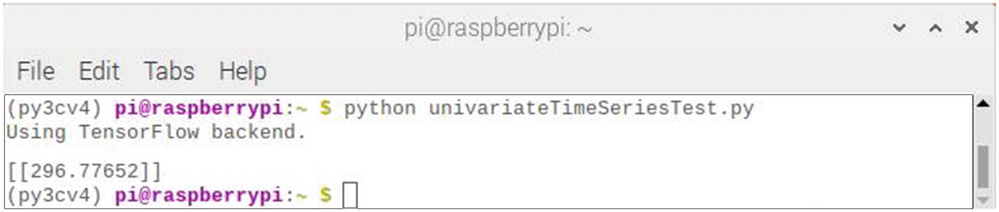
Figure 7-18
Results after running the univariateTimeSeriesTest script
The predicted value displayed is 296.78, not quite 300 as was expected, but still fairly close. There is a degree of randomness in the algorithm, and I tried running it a few more times. The following list shows the results of ten retries:
- 286.68
- 276.35
- 279.15
- 299.96
- 279.66
- 299.86
- 300.07
- 281.75
- 294.20
- 300.09
You can see from the list that the expected value (rounded) was displayed four out of ten times. The mean of the ten values was 289.78, the standard deviation was 10.03, and range was from 276.35 to 300.09. I would rate this CNN predictor as good with those performance statistics.
Multivariate time series CNN model
A multivariate time series is the same as a univariate time series except that there is more than one sampled value for each time step. There are two model types that handle multivariate time series data:
- Multiple input series
- Multiple parallel series
Each model type will be discussed separately.
Multiple input series
I will start by explaining that multiple input series has parallel input time series, which is not to be confused with the other model type. This will be clear in a moment. This parallel time series has had its values sampled at the sample time step. For example, consider the following sets of raw time series values:
- [50, 100, 150, 200, 250, 300, 350, 400, 450, 500, 550, 600, 650]
- [50, 75, 100, 125, 150, 175, 200, 225, 250, 275, 300, 325, 350]
The output sequence will be the sum of each sampled value pair for the entire length of each series. In code the aforementioned would be expressed as
from numpy import array
in_seq1 = array([50, 100, 150, 200, 250, 300, 350, 400, 450, 500, 550, 600, 650])
in_seq2 = array([50, 75, 100, 125, 150, 175, 200, 225, 250, 275, 300, 325, 350])
out_seq = array([in_seq1[i] + in_seq2[i] for i in range(in_seq1))])
These arrays must be reshaped as was done in the previous demonstration. The columns must also be stacked horizontally for processing. The code segment to do all that is
# Convert to [rows, columns] structure
in_seq1 = in_seq1.reshape((len(in_seq1), 1))
in_seq2 = in_seq2.reshape((len(in_seq2), 1))
out_seq = out_seq.reshape((len(out_seq), 1))
# Horizontally stack columns
dataset = hstack((in_seq1, in_seq2, out_seq))
Preprocessing the dataset
The complete script to preprocess the datasets described earlier is named shapeMultivariateTimeSeries.py and is listed in the following. It is available from the book’s companion web site.
# Multivariate data preparation
from numpy import array
from numpy import hstack
# Define input sequences
in_seq1 = array([50, 100, 150, 200, 250, 300, 350, 400, 450, 500, 550, 600, 650])
in_seq2 = array([50, 75, 100, 125, 150, 175, 200, 225, 250, 275, 300, 325, 350])
out_seq = array([in_seq1[i]+in_seq2[i] for i in range(len(in_seq1))])
# Convert to [rows, columns] structure
in_seq1 = in_seq1.reshape((len(in_seq1), 1))
in_seq2 = in_seq2.reshape((len(in_seq2), 1))
out_seq = out_seq.reshape((len(out_seq), 1))
# Horizontally stack columns
dataset = hstack((in_seq1, in_seq2, out_seq))
# Display the datasets
print(dataset)
Run this script by using this command:
python shapeMultivariateTimeSeries.py
Figure 7-19 shows the result of running this script.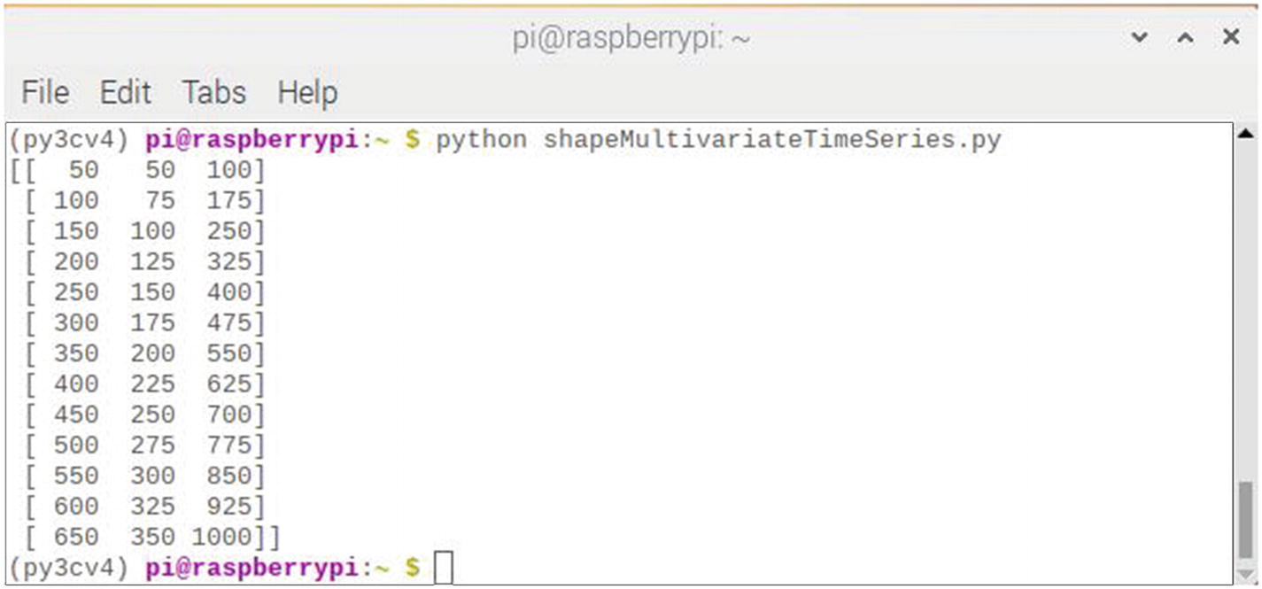
Figure 7-19
Results after running the shapeMultivariateTimeSeries script
The results screen shows the dataset with one row per time step and columns for the two inputs and summed output for each of the elements in the parallel time series.
This reshaped raw data vectors now must be split into input/output samples as was done with the univariate time series. A 1D CNN model needs sufficient inputs to learn a mapping from an input sequence to an output value. The data needs to be split into samples maintaining the order of observations across the two input sequences.
If three input time steps are chosen, then the first sample would look as follows:
Input:
- 50, 50
- 100, 75
- 150, 100
Output:
- 250
The first three time steps of each parallel series are provided as input to the model, and the model associates this with the value in the output series at the third time step, in this case, 250.
It is apparent that some data will be discarded when transforming the time series into input/output samples to train the model. Choosing the number of input time steps will have a large effect on how much of the training data is eventually used. A function named split_sequences will take the dataset that was previously shaped and return the needed input/output samples. The following code implements the split_sequences function
:
# split a multivariate sequence into samples
def split_sequences(sequences, n_steps):
X, y = list(), list()
for i in range(len(sequences)):
# find the end of this pattern
end_ix = i + n_steps
# check if we are beyond the dataset
if end_ix > len(sequences):
break
# gather input and output parts of the pattern
seq_x, seq_y = sequences[i:end_ix, :-1], sequences[end_ix-1, -1]
X.append(seq_x)
y.append(seq_y)
return array(X), array(y)
The following code tests all the previous code snippets and functions. I named this script splitMultivariateTimeSeries.py. It is available from the book’s companion web site.
# Import required libraries
from numpy import array
from numpy import hstack
# Split a multivariate sequence into samples
def split_sequences(sequences, n_steps):
X, y = list(), list()
for i in range(len(sequences)):
# find the end of this pattern
end_ix = i + n_steps
# check if we are beyond the dataset
if end_ix > len(sequences):
break
# gather input and output parts of the pattern
seq_x, seq_y = sequences[i:end_ix, :-1], sequences[end_ix-1, -1]
X.append(seq_x)
y.append(seq_y)
return array(X), array(y)
# Define input sequences
in_seq1 = array([50, 100, 150, 200, 250, 300, 350, 400, 450, 500, 550, 600, 650])
in_seq2 = array([50, 75, 100, 125, 150, 175, 200, 225, 250, 275, 300, 325, 350])
out_seq = array([in_seq1[i]+in_seq2[i] for i in range(len(in_seq1))])
# Convert to [rows, columns] structure
in_seq1 = in_seq1.reshape((len(in_seq1), 1))
in_seq2 = in_seq2.reshape((len(in_seq2), 1))
out_seq = out_seq.reshape((len(out_seq), 1))
# Horizontally stack columns
dataset = hstack((in_seq1, in_seq2, out_seq))
# Choose a number of time steps
n_steps = 3
# Convert into input/output samples
X, y = split_sequences(dataset, n_steps)
print(X.shape, y.shape)
# Display the data
for i in range(len(X)):
print(X[i], y[i])
Run this script by using this command:
python splitMultivariateTimeSeries.py
Figure 7-20 shows the result of running this script.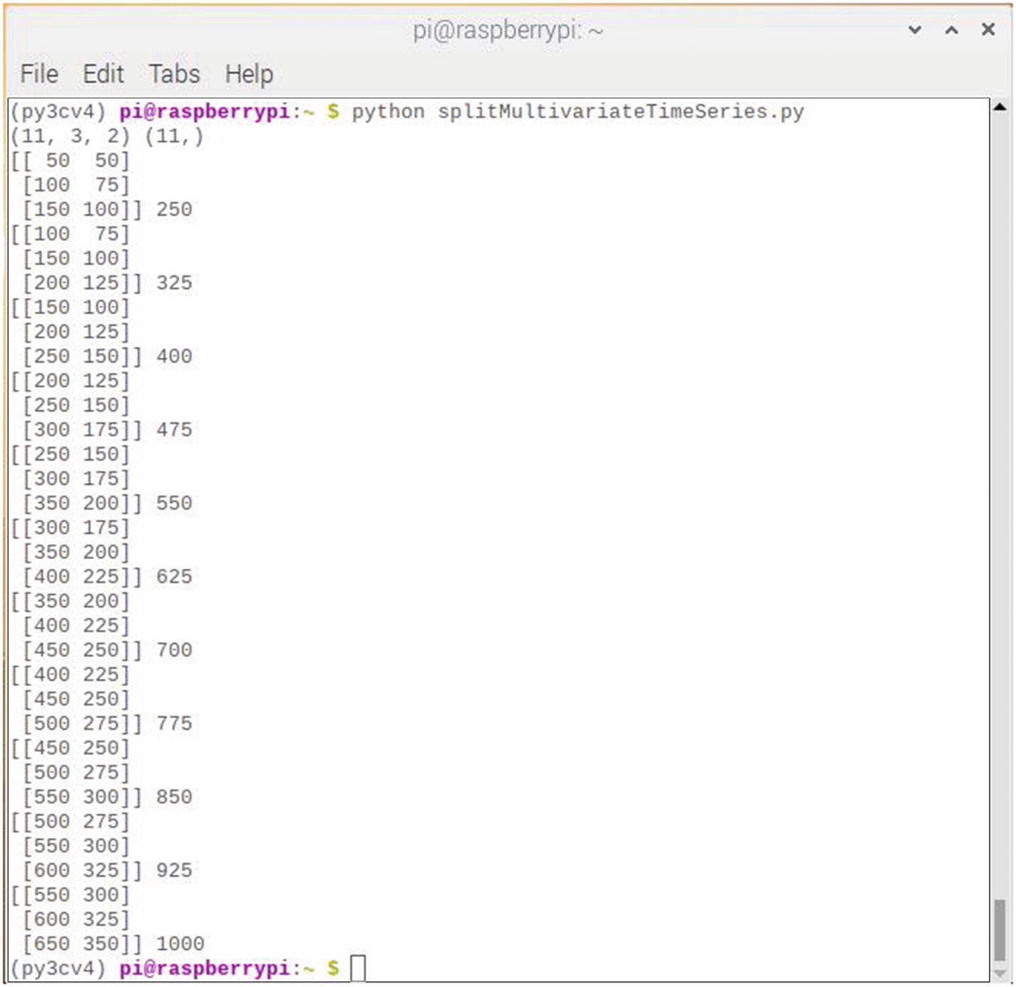
Figure 7-20
Results after running the splitMultivariateTimeSeries script
Running the script first displays the shape of the X and y components. You can see that the X component has a 3D structure. The first dimension is the number of samples, in this case 11. The second dimension is the number of time steps per sample, in this case 3, and the last dimension specifies the number of parallel time series or the number of variables, in this case 2, for the two parallel series. The dataset as shown in the rest of the figure is the exact 3D structure expected by a 1D CNN for input.
The model used for this demonstration is exactly the same one used for the univariate demonstration. The discussion I used for that model applies to this situation.
The Keras predict function will be used to predict the next value in the output series, provided the input values are
- 200, 125
- 300, 175
- 400, 225
The predicted value should be 625. The code for the prediction is
# Demonstrate prediction
x_input = array([[200, 125], [300, 175], [400, 225]])
x_input = x_input.reshape((1, n_steps, n_features))
yhat = model.predict(x_input, verbose=0)
The complete script incorporating all of the code snippets discussed earlier is named multivariateTimeSeriesTest.py and is listed in the following. It is available from the book’s companion web site.
# Import required libraries
from numpy import array
from numpy import hstack
from keras.models import Sequential
from keras.layers import Dense
from keras.layers import Flatten
from keras.layers.convolutional import Conv1D
from keras.layers.convolutional import MaxPooling1D
# Split a multivariate sequence into samples
def split_sequences(sequences, n_steps):
X, y = list(), list()
for i in range(len(sequences)):
# Find the end of this pattern
end_ix = i + n_steps
# Check if we are beyond the dataset
if end_ix > len(sequences):
break
# Gather input and output parts of the pattern
seq_x, seq_y = sequences[i:end_ix, :-1], sequences[end_ix-1, -1]
X.append(seq_x)
y.append(seq_y)
return array(X), array(y)
# Define input sequence
in_seq1 = array([50, 100, 150, 200, 250, 300, 350, 400, 450, 500, 550, 600, 650])
in_seq2 = array([50, 75, 100, 125, 150, 175, 200, 225, 250, 275, 300, 325, 350])
out_seq = array([in_seq1[i]+in_seq2[i] for i in range(len(in_seq1))])
# Convert to [rows, columns] structure
in_seq1 = in_seq1.reshape((len(in_seq1), 1))
in_seq2 = in_seq2.reshape((len(in_seq2), 1))
out_seq = out_seq.reshape((len(out_seq), 1))
# Horizontally stack columns
dataset = hstack((in_seq1, in_seq2, out_seq))
# Choose a number of time steps
n_steps = 3
# Convert into input/output samples
X, y = split_sequences(dataset, n_steps)
# The dataset knows the number of features, e.g. 2
n_features = X.shape[2]
# Define model
model = Sequential()
model.add(Conv1D(filters=64, kernel_size=2, activation="relu", input_shape=(n_steps, n_features)))
model.add(MaxPooling1D(pool_size=2))
model.add(Flatten())
model.add(Dense(50, activation="relu"))
model.add(Dense(1))
model.compile(optimizer='adam', loss="mse")
# Fit model
model.fit(X, y, epochs=1000, verbose=0)
# Demonstrate prediction
x_input = array([[200, 125], [300, 175], [400, 225]])
x_input = x_input.reshape((1, n_steps, n_features))
yhat = model.predict(x_input, verbose=0)
# Display the prediction
print(yhat)
Run this script by using this command:
python multivariateTimeSeriesTest.py
Figure 7-21 shows the result of running this script.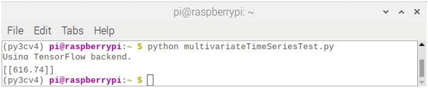
Figure 7-21
Results after running the multivariateTimeSeriesTest script
The predicted value displayed is 616.74.78, not quite 625 as was expected, but still reasonably close. There is a degree of randomness in the algorithm, and I tried running it a few more times. The following list shows the results of ten retries:
- 586.93
- 610.88
- 606.86
- 593.37
- 612.66
- 604.88
- 597.40
- 577.46
- 605.50
- 605.94
The mean of the ten values was 600.19, the standard deviation was 11.28, and range was from 577.46 to 612.66. I would rate this CNN predictor as fair to good with those performance statistics.