CHAPTER 4
Artificial Intelligence Techniques
Most of the trading strategies in this book are developed based on the process a theoretical physicist would use. Where a theoretical physicist develops a hypothesis, designs an experiment to test that hypothesis, and confirms the hypothesis based on the test results, we quantitative traders develop a hunch about a possible inefficiency in the market (e.g., retail investors' herd‐like behavior leading to stock momentum), devise a strategy to exploit that inefficiency, and use data to confirm whether that strategy actually works. The use of artificial intelligence (AI) or machine learning techniques is closer to the approach experimental physicists might take in their work: we don't have a preconceived theory of what the most important factors affecting the market are, and therefore, we need to explore as many factors and trading rules as possible with the help of efficient algorithms. Finance practitioners often derisively refer to this methodology as data mining. There is some justification of their derision: financial data are not only quite limited (unless we use tick data), they are also not very stationary in the statistical sense. That is, the probability distribution of returns does not stay constant forever. If we just turn our machine learning algorithms loose on these data, it is very easy to come up with trading rules that worked extremely well in certain past periods, but fail terribly going forward. Of course, even handcrafted trading models built with human intelligence can do that, too. But we can sometimes understand why it is that the model doesn't work anymore and take remedial actions. No such luck with machine‐learned rules.
Despite our cautiousness toward AI techniques, keep in mind that this is a rapidly advancing field, where practitioners are developing techniques specifically designed to avoid the overfitting bias we alluded to. One may remember that neural networks were dismissed as quite impractical just a few years ago, but a breakthrough made in 2006 (Allen, 2015) revitalized the field, and neural net experts are now much sought‐after in organizations such as Google and Facebook. More pertinent to trading, I remember a senior manager at the legendary quant fund Renaissance Technologies once remarked to the press that one of their most profitable trading strategies was also one that had no rational financial justification at all. That is also why it endured without being arbitraged away by other traders. These are the kind of trading rules that AI techniques can deliver to us. Another situation where AI techniques will be useful is when someone gives you a set of indicators, whether fundamental or technical, that you don't have any idea how to use and have no intuition about. Turning AI techniques loose on such indicators would be the easiest way to proceed. The results may even aid in gaining human understanding of the indicators. So let's not presume that our own minds and intuition have a monopoly on trading ideas and let AI surprise us!
The machine learning techniques we describe in this chapter are fairly basic and well‐known. That's why they have been encapsulated in commercial software packages and are easily accessible to traders who do not wish to reinvent the wheel or to become a full‐time AI researcher. The software packages that I use to demonstrate these techniques are MATLAB's Statistics and Machine Learning Toolbox and the Neural Network Toolbox, and in one instance, the Bayes Net Toolbox written by Dr. Kevin Murphy at Google. However, R programmers can easily find similar packages (Hothorn, 2014).
Though it may seem that we will be covering a hodgepodge of unrelated models, they can be categorized in several ways. Stepwise regression, regression tree, classification tree, support vector machine, and hidden Markov models can be considered linear models, or at least piecewise linear models, whereas a neural network is an explicitly nonlinear model. Stepwise regression, regression tree, and neural network typically try to predict response variables that are continuous, whereas classification tree and support vector machine try to predict responses that are discrete. (Hidden Markov models can work on either continuous or discrete data, but our example in this chapter is discrete.) All but the hidden Markov model use “supervised training” where we try to assign observable classes to data, whereas the hidden Markov model uses “unsupervised training” where we try to assign unobserved classes to the data.
All of these models can be improved by a number of common techniques. The first technique is called cross validation, where we train a lot of models on subsets of one training data set, and pick only the one that performs best out‐of‐sample. The second technique is called bagging. Here, we artificially create many training sets by resampling with replacement our original training set, and we train a model on each of these replicated training sets and average their predictions. The third technique is called random subspace, where instead of randomly sampling the training data as in bagging, we sample the predictors for each model that we create. The fourth technique, called random forest, is a hybrid between bagging and random subspace, and is especially designed for regression and classification trees. All four techniques are designed with the aim of reducing overfitting on the training set. There is a fifth technique that we will discuss, boosting, which is designed to force the learning algorithm to focus on its past prediction errors and improve on them.
To illustrate these models and techniques, we focus mostly on one simple example: the prediction of the ETF SPY's next‐day return based on its past returns with various lookback. This allows us to compare the efficacy and nuances of different models and techniques without the distraction of understanding a new data set for each new technique. This doesn't mean that SPY is the most favorable instrument for AI methods, of course. You are encouraged to try them out on your own favorite market. In fact, most of these techniques work better if we have more predictors, and we can readily find more fundamental variables than (uncorrelated) technical variables as predictors. Hence, we include one important example at the end to illustrate the application of one of these techniques to identifying predictive fundamental stock factors for returns prediction.
Since this is a book on practical trading, and not on the theoretical foundation of finance, much less the theoretical foundation of machine learning, we will not dwell on the intricate details of the algorithms presented here. Trading strategies based on AI have earned a well‐deserved reputation of being “black‐box.”1 Even if one were to understand fully the mathematical justification of every AI learning algorithm, we would be no closer to intuiting why the algorithm generates a certain trading signal at a certain moment.
Stepwise Regression
One key utility of AI is that an algorithm can automatically select the most important independent variables (predictors) for the prediction of a dependent (response) variable based on a model that specifies the functional relationship between them. For example, if we want to predict the future one‐day return of SPY, one predictor might be the previous one‐day return, another might be its stochastic oscillator (for a technical analyst), the third one might be its P/E ratio (for a fundamental analyst), and so on. We don't usually know which predictor is important, so we should just throw everything but the kitchen sink at the AI algorithm, and hope for the best. The AI algorithm will perform what is called feature selection. The model that relates the predictor to the response variables need not be complicated. In fact, we will begin with one of the simplest models—linear regression—to illustrate the AI paradigm. The result of marrying feature selection to linear regression is stepwise regression.
Let's look at the example predicting SPY returns. Instead of using a mixture of technical and fundamental predictors, let's just use previous returns with various lookbacks (1‐day, 2‐day, 5‐day, and 20‐day) as predictors. In a usual multiple regression, we would fit the future one‐day return to all the predictors simultaneously and find the regression coefficients of all the predictors (plus the y‐intercept.) This can be accomplished using the fitlm function in MATLAB:
model_train=fitlm([ret1(trainset) ret2(trainset) ret5(trainset) ret20(trainset)], retFut1(trainset), 'linear')
The ret1, ret2,…, ret20 are ![]() arrays with previous returns of various lookback, and retFut1 is a
arrays with previous returns of various lookback, and retFut1 is a ![]() array with the future one‐day return. By default, fitlm assumes there is a constant term, so we do not need to include a column of 1s in the predictors. The parameter “linear” indicates we don't want products of independent variables as predictors. We should not use the entire data set for fitting this regression model—we shall leave the second half of the data as the test set. Here trainset is an index array denoting the indices of the first half of the data. This separation between training and test sets is of course a procedure that we always follow in building any trading model, but especially important in building machine‐learning models due to their propensity for overfitting. To see how this model does on the training set as a sanity check, we apply the predict function to model and the training data:
array with the future one‐day return. By default, fitlm assumes there is a constant term, so we do not need to include a column of 1s in the predictors. The parameter “linear” indicates we don't want products of independent variables as predictors. We should not use the entire data set for fitting this regression model—we shall leave the second half of the data as the test set. Here trainset is an index array denoting the indices of the first half of the data. This separation between training and test sets is of course a procedure that we always follow in building any trading model, but especially important in building machine‐learning models due to their propensity for overfitting. To see how this model does on the training set as a sanity check, we apply the predict function to model and the training data:
retPred1=predict(model, [ret1(trainset) ret2(trainset) ret5(trainset) ret20(trainset)]);
retPred1 is similar to retFut1, but contains the predicted future one‐day returns instead of the actual future one‐day returns contained in retFut1. If we build a simple trading strategy by buying $1 of SPY when retPred1 is positive, and shorting $1 when it is negative, holding just one day:
positions(retPred1 > 0)=1;positions(retPred1 < 0)=-1;
we find that the CAGR is 34.3 percent, with a Sharpe ratio of 1.4. So this model fits the training data from December 22, 2004, to September 15, 2009, quite well—so far, so good. We can repeat the same procedure on the test data from September 16, 2009, to June 2, 2014. Running
retPred1=predict(model, [ret1(testset) ret2(testset) ret5(testset) ret20(testset)]);
and applying the same simple trading strategy on the test set now yields a CAGR of 0.4 percent, with a Sharpe ratio of 0.1. This model2 does no better than random on the test set. This establishes an easy benchmark for stepwise regression to beat.
Stepwise regression differs from multiple regression in that it starts with just one “best” predictor based on some common goodness of fit criterion such as the sum of squared error (the default for MATLAB's stepwiselm function), Akaike information criterion (AIC), or Bayesian information criterion (BIC). Then the algorithm will try to add other predictors one at a time until the goodness of fit does not improve. Then it goes in reverse and tries to remove predictors one at a time, again stopping when the goodness of fit does not improve. In practice, to switch from using multiple regression to stepwise regression in MATLAB is as simple as switching the name of the function from lmfit to stepwiselm.
model=stepwiselm([ret1(trainset) ret2(trainset) ret5(trainset) ret20(trainset)], retFut1(trainset), 'Upper', 'linear')
The input parameter name/value pair “Upper” with its value “linear” indicates that we only want linear functions of the independent variables as predictors, not products of them.
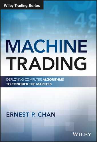
The algorithm picks just one predictor: ret2.3 This one predictor causes the in‐sample CAGR to go from 34.3 percent to 43.5 percent, and the Sharpe ratio from 1.4 to 1.6. This is unusually encouraging, because a simpler model with fewer predictors usually produces worse results than a complicated model in‐sample. But more importantly, stepwise regression causes the out‐of‐sample CAGR to go from 0.4 percent to 10.6 percent, and the Sharpe ratio from 0.1 to 0.7, indicating the model is close to achieving statistical significance (the threshold for that is a Sharpe ratio of 1). The equity curve shown in Figure 4.1 suggests that most of the performance comes during the earlier period from 2009 to 2011, but that isn't the fault of the algorithm. To improve on this, we can always retrain the program at every step by adding the latest data point to the training set. Also, the model makes a prediction of returns, but we have only used the sign of the return as a trading signal. One way to use the magnitude of the predicted return is to buy or sell only when the magnitude exceeds a certain threshold. Another way is to buy or sell a dollar amount that is proportional to the return magnitude. We will leave all these variations as exercises.
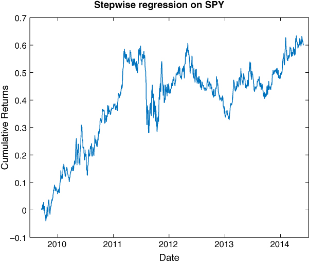
Figure 4.1: Out‐of‐sample performance of stepwise regression on SPY
One last detail we should notice: the regression coefficient of ret2 is negative, meaning that this model predicts that future one‐day return will revert from the past two‐day return. Just because a model is generated by AI doesn't mean that we should not use it to improve our own understanding of the market!
Regression Tree
Using a regression tree (and its sibling classification tree for discrete dependent variables such as, “Will it be an up or down day tomorrow?”) is another way one can select important predictors. However, unlike stepwise regression, where all the selected predictors are applied to all data jointly just as in a multiple regression, regression trees take a hierarchical approach. In fact, the regression tree algorithm has little to do with linear regression. Once the algorithm picks the “best” predictor based on some criterion, it will split the data into two subsets by applying an inequality condition on this predictor (such as “previous two‐day return ![]() 1.5%”). The original data form the parent node, and each subset is a child node. The algorithm will then be iteratively applied to each child node, until a stopping condition is met. The criterion that is used to pick the best predictor at each node is usually based on minimizing the variance of the response variable in each child node (Breiman et al., 1984). Minimizing the variance of the response variable in a node is another way of saying we want to minimize the mean squared error (MSE) of the predicted response compared to the true response, because the predicted response for a node is none other than the average of the response variables. The stopping condition is met when any of the following occur:
1.5%”). The original data form the parent node, and each subset is a child node. The algorithm will then be iteratively applied to each child node, until a stopping condition is met. The criterion that is used to pick the best predictor at each node is usually based on minimizing the variance of the response variable in each child node (Breiman et al., 1984). Minimizing the variance of the response variable in a node is another way of saying we want to minimize the mean squared error (MSE) of the predicted response compared to the true response, because the predicted response for a node is none other than the average of the response variables. The stopping condition is met when any of the following occur:
- There is no reduction of variances compared to the variance of the parent node; or
- There are too few observations in the parent node (MinParentSize is an input parameter); or
- Splitting the parent node using any predictor would have resulted in a child node with too few observations (MinLeafSize is another input parameter); or
- The maximum number of nodes have been reached (MaxNumSplits, a third input parameter, limits the total number of splits).
Note that due to the iterative nature of this algorithm, the same predictor can be reused at each child node for an unlimited number of times. Each “leaf” of a tree (a child node without children itself) can be summarized as a set of inequalities on the predictors (e.g., “previous two‐day return ![]() 1.5%” and “previous one‐day return
1.5%” and “previous one‐day return ![]() −1.4%”). We can therefore pick those leaves (equivalently, the set of inequalities) that have the average response (e.g., high average future one‐day return) we desire. When we have a new data point from the test set that satisfies all the inequalities that lead to a leaf with high average future return, we will predict that this data point will generate a high future return, too.
−1.4%”). We can therefore pick those leaves (equivalently, the set of inequalities) that have the average response (e.g., high average future one‐day return) we desire. When we have a new data point from the test set that satisfies all the inequalities that lead to a leaf with high average future return, we will predict that this data point will generate a high future return, too.

Figure 4.2: Regression tree on SPY
We can try our hands at the regression tree algorithm on the same set of data, predictors, and response variable (future one‐day return of SPY) as we used in the stepwise regression example. The program rTree.m is practically the same as stepwiseLR.m: we just need to replace the function stepwiselm with fitrtree.
model=fitrtree([ret1(trainset) ret2(trainset) ret5(trainset) ret20(trainset)], retFut1(trainset), 'MinLeafSize', 100);
We choose to set MinLeafSize to 100, but you are free to experiment with other values and see what is optimal on the trainset. Generally speaking though, we don't want to have a leaf size that is too small in order to avoid overfitting. To see what the tree looks like, including the inequalities in each child node, apply the function view to the model:
view(model, 'mode', 'graph'); % see the tree visually
which produces Figure 4.2.

Figure 4.3: Trading model based on regression tree
We can examine the numbers below the leaf nodes: they indicate the expected value of the response variable under the sequence of inequalities. For example, if we want a leaf node with the highest expected value (0.0047136 for the left‐most node), we see that the sequence is x2 < 0.015314, x1 < −0.00244162, x1 < −0.0139236, which we can paraphrase as ret2 < 1.53% and ret1 < −1.39%. This can be used as a ready‐made trading rule for buying SPY. Similarly, we can look for a leaf node with the most negative expected value (−0.004527 for the right‐most node). The single inequality that leads to that can be paraphrased as ret2 >= 1.53%. This can be used as a trading rule for shorting SPY. Both trading rules are mean‐reverting, just as the trading model produced by stepwise regression. If we buy SPY at the close and hold it one day according to the long rule, and short SPY and hold it one day according to the short rule, we obtain a CAGR of 28.8 percent with a Sharpe ratio of 1.5 on the training set, and a CAGR of 3.9 percent with a Sharp ratio of 0.5 on the test set. This isn't as good as the stepwise regression result, and the equity curve in Figure 4.3 also shows that these mean reversion models worked only during the first half of the test set.
One may wonder why we limit ourselves to the two extreme leaves (extreme in terms of expected response), and do not generate a trading rule based on the expected response of every single leaf? If we try that (all we need to do is to use the predict function we have used before in stepwiseLR.m.), we will find that the in‐sample CAGR will be boosted to 73 percent, but the out‐of‐sample CAGR will drop to −7.2 percent—a clear symptom of overfitting. But there is a way to have your cake and eat it, too. In the next three sections, we will explore some general techniques for reducing overfitting so that we can in fact use all leaves for prediction.

Figure 4.4: Leaving out a subset of training set for cross‐validation test
Cross Validation
Cross validation is a technique for reducing overfitting by testing for out‐of‐sample performance as part of model building. To do this, we randomly divide the training set into K roughly equal subsets. Model i will be built on the union of all subsets except the ith. We then test for the predictive accuracy of model i on the out‐of‐sample ith part. (See Figure 4.4.) This is called the cross‐validation accuracy. Finally, we will pick the model that has the highest cross‐validation accuracy.
We can try this on the regression tree model we built in the previous section that uses every leaf for generating trading signals. We simply need to add the name/value pairs “CrossVal” and “On,” “KFold” and 5, when using fitrtree for model building. This would generate ![]() trees stored in model_cv below:
trees stored in model_cv below:
model_cv=fitrtree([ret1(trainset) ret2(trainset) ret5(trainset) ret20(trainset)], retFut1(trainset), 'MinLeafSize', 100, 'CrossVal', 'On', 'KFold', 5);
To find the cross‐validation accuracy (or its inverse, the loss or mean squared error of the predicted responses compared to the true responses) of each tree, we apply the kfoldLoss function to these trees and pick the tree with the minimum loss:
L= kfoldLoss(model_cv,'mode','individual'); % Find the loss (mean squared error) of the predicted responses in a fold when compared against predictions made with a tree trained on the out-of-fold data.[~, minLidx]=min(L); % pick the tree with the minimum loss, i.e. with least overfitting error.bestTree=model_cv.Trained{minLidx};
Running the predict function on the test set using bestTree as the model generates a CAGR of 0.6 percent with a Sharpe ratio of 0.11, which is definitely better than the previous result without using cross validation, but not as good as if we just pick the two extreme leaves. (If you run this program with a different random seed, you will get a different tree and different CAGR. This is because the cross‐validation algorithm picks the subsets of training data for each tree randomly.) The code for this is part of rTree.m.
Some readers may wonder why we pick ![]() instead of 10, which is the MATLAB default for the number of subsets used for cross validation. The reason is that while our training set from December 22, 2004, to September 15, 2009, may be a reasonable size for trading research, it is considered quite small by machine learning standards. If we divide this training set into 10 subsets, the out‐of‐sample subset will be so small that the cross‐validation accuracy is subject to large statistical errors, and so the “best” tree produced won't necessarily be any good when applied to the test set. On the other hand, if we set K to be too small, say 2, then we don't have enough trained models to choose the best one from.
instead of 10, which is the MATLAB default for the number of subsets used for cross validation. The reason is that while our training set from December 22, 2004, to September 15, 2009, may be a reasonable size for trading research, it is considered quite small by machine learning standards. If we divide this training set into 10 subsets, the out‐of‐sample subset will be so small that the cross‐validation accuracy is subject to large statistical errors, and so the “best” tree produced won't necessarily be any good when applied to the test set. On the other hand, if we set K to be too small, say 2, then we don't have enough trained models to choose the best one from.
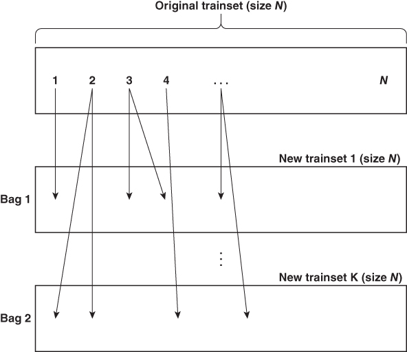
Figure 4.5: Bagging with K bags (In bag 1, data samples 2 and 4 will be part of test set 1. In bag K, data samples 1 and 3 will be part of test set K.)
Bagging
In cross validation, we introduced the idea that it is often useful to present somewhat different training data sets to the learning algorithm so that it does not overfit to the statistical fluctuations in one single training set that won't be repeated in the test set. Bagging is another variation on this theme. Instead of randomly dividing the original training set of size N into subsets as we did in cross validation, we randomly sample N observations from the original training set with replacement to form a replica (a bag) of the original training set. Since we are sampling with replacement, some observations from the original training set will be repeated multiple times in the replica and other observations will be omitted (these will be called out‐of‐bag observations). We repeat this process K times, so that we form an ensemble of K such replicas, each with the original training set size N. Since this process essentially increases the training sample size, it is also called bootstrapping. Like cross validation, we will train a model (regression tree in our example) on each replica, and test its predictive accuracy on the corresponding out‐of‐bag (and, therefore, out‐of‐sample) observations. (See Figure 4.5.) But unlike cross validation, we do not just pick the tree with the most accurate out‐of‐bag prediction. We average the predicted response from all the trees built from all the replicas.
To apply bagging to the regression tree learner, use the TreeBagger instead of the fitrtree function in MATLAB:
model=TreeBagger(5, [ret1(trainset) ret2(trainset) ret5(trainset) ret20(trainset)], retFut1(trainset), 'Method', 'regression', 'MinLeaf', 100);
We picked K = 5 (the first parameter in the TreeBagger function4) since this was the number of trees we built with cross validation as well. This yielded significantly better predictive performance than the cross validation model: CAGR is 7.2 percent with a Sharpe ratio of 0.5. The equity curve is displayed in Figure 4.6.
Figure 4.6: Trading model based on regression tree with bagging (K = 5)
Increasing ![]() will actually degrade out‐of‐sample performance, because the average result of a large ensemble of replicas will be very similar to that of using the original training set.
will actually degrade out‐of‐sample performance, because the average result of a large ensemble of replicas will be very similar to that of using the original training set.
Random Subspace and Random Forest
With bagging, we randomly sample data with replacement to train multiple models. With random subspace, we randomly sample predictors with replacement (but with decreasing sampling probability for those that have been chosen previously) to train multiple models. In both cases, we will average the predictions of all these models (weak learners) so that the ensemble prediction is stronger. Any method that trains many weak learners to form a strong learner is called an “ensemble” method.
In MATLAB, the function that implements random subspace is fitensemble, if we set the “Method” variable to “Subspace.” However, it only works on classification problems (i.e., with discrete instead of continuous response variables). We will discuss that in the section on “Classification Tree.” Also, the random subspace method really shines only when we have a large number of predictors, so we won't be able to demonstrate it here using our SPY example even if we were to discretize the response variable. Instead, we invite you to try it as an exercise using the fundamental data set suggested in the section “Application to Stocks Selection.”
There is another ensemble method called random forest that is a hybrid of bagging and random subspace. More specifically, a random forest is a regression or classification tree where we start with a randomly selected (with replacement) subset of training data, and at each split of the node, choose the best predictor from a randomly selected (with replacement) subset of all the available predictors. Again, we will average the prediction of the weak learners. In MATLAB, random forest is implemented using the TreeBagger function, with the “NumPredictorsToSample” parameter set to any number smaller than the total number of predictors. Actually, the MATLAB default is to have NumPredictorsToSample set to one‐third of the total number of predictors, which is what we used in the bagging example in the previous section and in rTreeBagger.m. If we actually want to use all the predictors at every node for prediction, we can set NumPredictorsToSample to “all.” This decreases the out‐of‐sample CAGR of the previous example from 7.2 percent to 1.5 percent, and the Sharpe ratio from 0.5 to 0.2.
Boosting
As humans, we pride ourselves on our ability to learn from our past mistakes. The best of us don't waste our time reminiscing on past triumphs. It turns out that we can teach our AI algorithms to do the same, and this method is called boosting.
Boosting involves applying a learning algorithm iteratively to the prediction errors of the model constructed in the previous iteration. As a first step in boosting, we apply a learning algorithm such as a regression tree to the training data as before. The first step is complete once the tree is constructed and predictions made for the training set. We begin the second step by creating a new training set where the responses are the differences between the actual responses and the predicted response from the first model. The objective of this second tree is to minimize the square of these differences. We will repeat this so as to create a total of M trees and take the predictions of the Mth tree as final. The hope is again to turn a weakly predictive algorithm into a stronger one.

Figure 4.7: Effect of boosting a regression tree on train vs. test set Sharpe ratio
We will apply this procedure to the regression tree model that we created before. We need to just replace fitrtree function with the fitensemble function in our code (rTreeLSBoost.m), just as in the case with the random subspace method. We need to specify “LSBoost” as the boosting algorithm, which is the gradient descent method (Friedman, 1999) for boosting regression or regression tree models. We also specify M as the number of iterations for boosting. Finally, we specify “Tree” as the learning algorithm.
model=fitensemble([ret1(trainset) ret2(trainset) ret5(trainset) ret20(trainset)], retFut1(trainset), 'LSBoost', M, 'Tree');
As opposed to cross validation and bagging, boosting does not seem to alleviate overfitting (although there are theoretical arguments on why it won't overfit). (See Kun, 2015.) We can see in Figure 4.7 the effect of boosting the previously constructed regression tree on the train versus test set. With increasing number of iterations, the Sharpe ratio on the trainset increases rapidly, while the Sharpe ratio on the test set increases much more slowly. In fact, the Sharpe ratio for the test set remains insignificant at any reasonable number of iterations. Applying cross validation to the best tree at each iteration actually worsens performance.
Classification Tree
The core learning algorithms we have discussed so far assume that the response variable is continuous. This is natural because we are mostly interested in expected returns in trading. But there are some learning algorithms that are specifically designed for discrete (also called categorical) response variables. There is no reason why we should deprive ourselves of them—we just need to discretize our returns into, say, positive and negative returns. In this section, we will apply the classification tree to the SPY prediction task.
Classification tree is a close sibling of regression tree. With regression tree, the best predictor to split a node is one that minimizes variance of responses in the child nodes. With classification tree, the variance of responses is replaced by the analogous Gini's Diversity Index (GDI). For a binary classification into positive (+) or negative (−) classes, GDI for a node is
where ![]() is the fraction of observations with positive returns, and
is the fraction of observations with positive returns, and ![]() is the fraction of observations with negative returns. GDI has a minimum value of zero, which is obtained when the node consists of observations of the same class—that is, perfect classification. The best predictor to split a node is one that minimizes the sum of the GDIs of both child nodes. Naturally, the predicted response of a node is the observation that constitutes the highest fraction.
is the fraction of observations with negative returns. GDI has a minimum value of zero, which is obtained when the node consists of observations of the same class—that is, perfect classification. The best predictor to split a node is one that minimizes the sum of the GDIs of both child nodes. Naturally, the predicted response of a node is the observation that constitutes the highest fraction.
To implement classification tree in MATLAB, simply replace the function fitrtree in our program rTree.m with fitctree, taking care to discretize the response variable.5 Since we know that using the entire tree for prediction suffers from severe data snooping bias, we will also impose fivefold cross validation as we did with regression trees:
model=fitctree([ret1(trainset) ret2(trainset) ret5(trainset) ret20(trainset)], retFut1(trainset)>= 0, 'MinLeafSize', 100, 'CrossVal', 'On', 'KFold', 5); % Response: True if>=0, False if < 0.
We can use this model in an obvious way to generate trading signal: just buy when the predicted response is positive, and short when it is negative. The complete program is in cTree.m. The resulting CAGR on the test set is 4.8 percent, with a Sharpe ratio of 0.4, which is better than the cross‐validated regression tree results, but not as good as the regression tree with random forest. (Of course, you can apply the random forest algorithm to the classification tree as well. This is left as an exercise.)

Figure 4.8: Support vector machine illustrated
One doesn't have to categorize the response as positive or negative returns. We can create a class for high positive returns (i.e., returns higher than some threshold) and another one for the complement, and generate buy signals only when we predict this high‐return class. Similarly, we can create a class for low negative returns and generate short signals for predictions in this class. However, this doesn't seem to improve the performance of the trading strategy.
Support Vector Machine
The support vector machine (SVM) is another popular classification technique that works on discrete responses. The intuitive idea behind it is quite visually appealing: let's imagine each sample data point resides in an m‐dimensional space, where m is the number of predictors (which are still continuous variables). Let's say some of these data points are labeled “plus” the remaining ones are labeled “minuses.” (See Figure 4.8). These pluses and minuses are our discrete responses. The SVM attempts to find a hyperplane in this m‐dimensional space that can separate the pluses from the minuses. Furthermore, it wants to separate them with the largest possible margin. If that can be done, we have achieved our classification task: whenever a data point has coordinates on one side of this hyperplane, we will know exactly which response category it will have. In our 2‐D illustration in Figure 4.8, the black line in the middle achieves such a clean separation: all the minuses are on the right side of the line, and all the pluses are on the left. The pluses that come closest to the separating hyperplane (line) form a set of “support vectors,” and so do the minuses that come closest. The separation between the two sets of support vectors is the margin which we maximized with our SVM.
Of course, real data are rarely as obliging as our fantasy data set. Even with the “best” hyperplane, we will find pluses on the right side and minuses on the left. We can attempt to find the best hyperplane by maximizing the margin of separation while simultaneously minimizing a penalty term that penalizes misclassified data points. (The mathematical details can be found in Anonymous, 2015.) To use the SVM in MATLAB, simply substitute the function fitcsvm for fitctree and again apply fivefold cross validation.6
model=fitcsvm([ret1(trainset) ret2(trainset) ret5(trainset) ret20(trainset)], retFut1(trainset)>= 0, 'CrossVal', 'On', 'KFold', 5); % Response: True if>=0, False if < 0.
The resulting CAGR of 13.3 percent with a Sharpe ratio of 0.8 on the test set is much superior to that of the classification tree. The equity curve in Figure 4.9 also shows no deterioration in the more recent period. This outperformance is perhaps because the model resulting from this basic version of the SVM is genuinely linear: after all, it is just a hyperplane. (The classification tree can be thought of as piece‐wise linear only.) Linear models avoid overfitting and generate better results on out‐of‐sample data. Interestingly, this same linear model performs worse on the training set, perhaps for the same reason.

Figure 4.9: Support vector machine with cross validation
Sometimes, however, we do need to transform predictors nonlinearly before the SVM is able to classify the data. These transformations are carried out by the Kernel function. Instead of a linear Kernel function, we can specify a polynomial function. Instead of setting the Kernel scale to 1, we can specify “auto” such that the algorithm will select an optimal Kernel scale. We have tried this new configuration, and the results weren't improved. If we try the radial basis (Gaussian) function, the results are slightly improved. There is also a multilayer perceptron (sigmoidal) function that we can apply, but it isn't part of the Statistics and Machine Learning Toolbox, so you would have to construct it yourself. (Interested readers can explore whether they can extract this function from the Neural Network Toolbox and apply that to the SVM.) Applying a nonlinear Kernel function to the predictors is effectively using a curved membrane instead of a plane to cut through the data. Another way of thinking about the Kernel transformation is that we are transforming the data into a higher dimensional space such that a hyperplane there can cleanly separate them. A reverse transformation of this hyperplane appears as a curve, not a line, in the original space. This allows for much more flexibility (and more room for overfitting).
Hidden Markov Model
It is common for traders to label a certain market moment “bull” or “bear.” It isn't clear, though, what constitutes a bull or bear market, since we can certainly experience down days in a bull market and up days in a bear market. No two cable TV commentators are able to agree on the exact definition of a bull or bear market. The same goes for “mean‐reverting” versus “trending” markets, or “risk‐on” versus “risk‐off” regimes. Machine learners, however, are quite accustomed to such ambiguity. More precisely, they are accustomed to classification problems where the classes are not actually observable, unlike the “up” or “down” days that we asked the SVM to classify in the previous section. Such classification of unobservable (hidden) states are the domain of “unsupervised learning” methods.
One of the most well‐known models with hidden states is the Hidden Markov Model (HMM). The easiest way to understand an HMM is to imagine that bull versus bear markets are two hidden states, and a transition probability matrix describes the probabilities that the market would jump from one state to another from one day to the next. For example, if we label the bull market as the first state, and bear market as the second, a transition matrix ![]() such as
such as

indicates that there is a probability of 0.6 that a bull market will remain so the next day. Of course, that also implies it has a probability of 0.4 to transition to a bear market. This matrix also indicates there is a probability of 0.25 that a bear market will remain so the next day, and a probability of 0.75 that it will transition to a bull market. Naturally, the probabilities on each row must add up to 1.
Besides the transition probabilities as tabulated in the transition matrix, we also need to know the probabilities that a bear state will “emit” a down day and an up day, respectively. The down and up days are called emissions, or observables. Similarly, we need to know the same for a bull state. These “emission” probabilities are tabulated in an emission probability matrix ![]() such as
such as

where we label the down days as the first emission symbol and the up days as the second. So this emission matrix is telling us that there is a 19 percent chance that a bull state will emit a down day, and an 81 percent chance that it will emit an up day. There is a 97 percent chance that a bear state will emit a down day and a 3 percent chance that it will emit an up day. Again, the probabilities of each row must sum to one. Figure 4.10 illustrates the transition matrix.
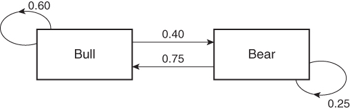
Figure 4.10: Hidden states transition probabilities of an HMM
Since bull and bear are unobservable, they are just names we give to the states. They can just as well be called “mean‐reverting” and “trending,” or “risk‐on” and “risk‐off,” or even “greed” and “fear,” and the learning algorithm will be none the wiser. The only assumption we have made is that the down and up days are generated by two unobservable states, in order to account for the fact that the probabilities of observing the up and down days seem not to be described satisfactorily by a stationary probability distribution. In other words, we can regard HMM as just a more complicated time‐series model than the ones we described in Chapter 3, with more parameters to estimate, and needless to say, more scope for data‐snooping bias.
Just like other learning algorithms, the parameters (namely, the transmission matrix ![]() and the emission matrix
and the emission matrix ![]() , and possibly the prior probability distribution on the emissions) need to be estimated using the training set. One of the most famous unsupervised learning algorithms for an HMM, and indeed for any models with hidden states, is the EM algorithm (Murphy, 2012). Mathworks' Statistics and Machine Learning Toolbox does have the function hmmtrain that implements a version of the EM algorithm, but unfortunately, it often returns singular solutions for unbeknownst reasons. Instead, we used an open‐source software called Bayes Net Toolbox for MATLAB (https://code.google.com/p/bnt/) for training. This is a complex piece of software, and quite difficult to use. We used their function called learn_params_dbn_em for training, as shown in our program hmm_train.m. The goal of training is, as usual, to find the parameters that generate the maximum log likelihood of the emissions. Since I expect there will be multiple local maxima, I run this training process 10 times, record the likelihood achieved for each maximum, and pick the model that has the highest likelihood among them. (Of course, if your computer is much faster than mine, or if you have much more patience than I did, you can run this many more times than 10.) Running this on SPY daily returns gives the T and E matrices that I used previously.
, and possibly the prior probability distribution on the emissions) need to be estimated using the training set. One of the most famous unsupervised learning algorithms for an HMM, and indeed for any models with hidden states, is the EM algorithm (Murphy, 2012). Mathworks' Statistics and Machine Learning Toolbox does have the function hmmtrain that implements a version of the EM algorithm, but unfortunately, it often returns singular solutions for unbeknownst reasons. Instead, we used an open‐source software called Bayes Net Toolbox for MATLAB (https://code.google.com/p/bnt/) for training. This is a complex piece of software, and quite difficult to use. We used their function called learn_params_dbn_em for training, as shown in our program hmm_train.m. The goal of training is, as usual, to find the parameters that generate the maximum log likelihood of the emissions. Since I expect there will be multiple local maxima, I run this training process 10 times, record the likelihood achieved for each maximum, and pick the model that has the highest likelihood among them. (Of course, if your computer is much faster than mine, or if you have much more patience than I did, you can run this many more times than 10.) Running this on SPY daily returns gives the T and E matrices that I used previously.
For prediction, we return to Mathworks' Statistics Toolbox. We need the function hmmdecode, which computes the probabilities of the hidden states from the initial time up to time t and stores them as ![]() . These probabilities are computed given known transmission and emission matrices and conditioned on our knowledge of the observed emissions data stored in a
. These probabilities are computed given known transmission and emission matrices and conditioned on our knowledge of the observed emissions data stored in a ![]() vector. To predict the emission at time
vector. To predict the emission at time ![]() , we need to know
, we need to know ![]() , which is given by
, which is given by ![]() , where
, where ![]() is the transpose of
is the transpose of ![]() . Then the probabilities of emissions are
. Then the probabilities of emissions are  . The MATLAB code fragment for this is
pemis=NaN(2, size(data, 1));for t=1:size(data, 1)-1[pstates]=hmmdecode(data(1:t)', T, E);pemis(:, t+1)=E'*T'*pstates(:, end);end
Note that this algorithm requires us to run hmmdecode with all previously observed data as input. It is not an “online” algorithm where we can just add the latest data point at time t and it would update ![]() . In contrast, the continuous sibling of HMM is the Kalman filter, where we have indeed used an online algorithm to update our estimates of the hidden state variable and other parameters in our discussion in Chan (2013) and again mentioned in Chapter 3 of this book. We will leave the task of finding (or implementing one from scratch) an online decoding function for HMM as an exercise.
. In contrast, the continuous sibling of HMM is the Kalman filter, where we have indeed used an online algorithm to update our estimates of the hidden state variable and other parameters in our discussion in Chan (2013) and again mentioned in Chapter 3 of this book. We will leave the task of finding (or implementing one from scratch) an online decoding function for HMM as an exercise.
Given the emission probabilities for the next day, we can construct a simple trading strategy that buys SPY if the probability of “up” is higher than “down,” and vice versa. We have created the program hmm_test.m to do just that. For the training set, it performed decently, giving a CAGR of 8.7 percent, but it gives a CAGR of 1 percent for the test set.
There are many variations to the way we builds an HMM to predict the next day return. Instead of estimating parameters using the first half of the data as training set, we can perform estimation with every new observed emission. Instead of discrete emissions (up or down days), we can model them as continuous variables with some parametric distributions such as Gaussian or Student‐t (Dueker, 2006). Instead of the emissions depending only on the hidden state variables, they can depend on some observed input variables too (such as the predictors used in all the supervised models in this chapter so far).
There is a side benefit of using HMM, aside from using it to predict the next emission. Given the observed emissions, HMM can tell us what the most probable hidden state sequence is. We can use the hmmviterbi function for that (in honor of Prof. Andrew Viterbi, the inventor of the decoding algorithm and the cofounder of Qualcomm, Inc., which likely made the chip in your smartphone).
states=hmmviterbi(data, T, E);
What is the benefit of knowing the most probable state sequence? Next time, if someone asks you whether you think this is a bull or bear market, you can consult your HMM and give them a well‐defined answer.7
Neural Network
Neural network may be the most well‐known of the machine learning algorithms. Because of its long history, it has also evolved into many subspecies, architectures, and training algorithms. It is in fact so evolved that Mathworks decided to gather all neural network algorithms into a separate Neural Network Toolbox. We certainly won't be able to do justice to all its flavors in a few short paragraphs. Instead, we will highlight the most basic architecture that is suitable for our SPY returns prediction task.
We can understand neural network as simply a way to approximate any function of an arbitrary number of predictor variables by a linear function of sigmoid functions ![]() , or linear function of sigmoid functions of linear functions of sigmoid functions, and so on. How many iterations of these sigmoid functions to use, how much weight to put on each, how to connect the output of one such function to the input of another, can only be decided by experimentation and optimization on the training set. Determining the weight of each function based on the training data set is the job of the training algorithm, which is also an optimization problem on the training set.
, or linear function of sigmoid functions of linear functions of sigmoid functions, and so on. How many iterations of these sigmoid functions to use, how much weight to put on each, how to connect the output of one such function to the input of another, can only be decided by experimentation and optimization on the training set. Determining the weight of each function based on the training data set is the job of the training algorithm, which is also an optimization problem on the training set.
The most basic architecture we can use is the feed forward network. A feed forward network consists of a number of hidden layers, each with a number of “neurons” that represent the sigmoid functions (with different weights), and a final output layer that represents a linear function. In the Neural Network Toolbox, the number of neurons in each layer can be specified as an input parameter hiddenSizes (a row vector) to the feedforwardnet function. For example, we can specify
hiddenSizes=[2 4 3];
which indicates the first layer has 2 neurons, the second 4 neurons, and the third 3. This means that our input vector ![]() , which in the SPY example has a dimension of 4, plus the constant 1 just like the constant offset of a linear regression, is first summed into a scalar with different weights:
, which in the SPY example has a dimension of 4, plus the constant 1 just like the constant offset of a linear regression, is first summed into a scalar with different weights:

where ![]() is the input to the
is the input to the ![]() neuron, and
neuron, and ![]() is the weight (to be determined during the training phase of the network) for the
is the weight (to be determined during the training phase of the network) for the ![]() component of the input vector for the
component of the input vector for the ![]() neuron, and
neuron, and ![]() is its constant offset. The output of each of these two linear functions of the input is then fed into its corresponding sigmoid function.
is its constant offset. The output of each of these two linear functions of the input is then fed into its corresponding sigmoid function.

Figure 4.11: A feed forward neural network for our example
If the sigmoid function were just the identity function ![]() , this neuron would be just our usual multiple linear regression fit discussed in the beginning of the section on stepwise regression. But instead, we believe a nonlinear function will fit better, and thus neural networks use the sigmoidal form shown before. The output of the two first layer neurons is a vector
, this neuron would be just our usual multiple linear regression fit discussed in the beginning of the section on stepwise regression. But instead, we believe a nonlinear function will fit better, and thus neural networks use the sigmoidal form shown before. The output of the two first layer neurons is a vector ![]() with a dimension of 2, which is then fed as input into each of four neurons in the second layer, and so on. Finally, the output of the final three neurons in the third layer is then fed as a three‐vector into the output layer with just one node, this time just a linear function. This assumes, as in our example, that the output is a scalar
with a dimension of 2, which is then fed as input into each of four neurons in the second layer, and so on. Finally, the output of the final three neurons in the third layer is then fed as a three‐vector into the output layer with just one node, this time just a linear function. This assumes, as in our example, that the output is a scalar ![]() . If the output is a vector, then there will be several nodes in the output layer corresponding to the dimension of the output vector. This sequence of iterated operations on an input vector: multiplication by weights (
. If the output is a vector, then there will be several nodes in the output layer corresponding to the dimension of the output vector. This sequence of iterated operations on an input vector: multiplication by weights (![]() ), summation of different components (
), summation of different components (![]() ), and transformation by the sigmoid function (
), and transformation by the sigmoid function (![]() ), is represented by the network diagram in Figure 4.11.
), is represented by the network diagram in Figure 4.11.
Instead of starting with all these hidden layers and multiple neurons for our SPY return prediction problem, let's just start with one hidden layer with one neuron (hiddenSizes = 1). Overfitting is a paramount concern, as always, and more hidden layers with more neurons make things worse. We will not discuss the training algorithm for the weights (w), except to note that there is randomness involving the initial guesses of the weights, and these different guesses will cause the final network to settle onto different local minima in network prediction error on the trainset. To minimize overfitting, the training algorithm utilizes a cross validation data set, whose size is specified by the user:
net.divideParam.trainRatio=0.6; % 0.6 (default is 0.7) Pick 4/5 of trainset randomly to serve as train datanet.divideParam.valRatio=0.4; % 0.4 (default is 0.15) Pick 1/5 of remaining trainset to serve as validation data for early stoppingnet.divideParam.testRatio=0;
where trainRatio indicates the percentage of the training data set we will randomly pick for prediction error minimization, valRatio indicates the percentage of the validation set, and testRatio is the percentage of the test set. If during network training, the error on the validation set starts to increase, training will stop immediately. We set the test set to zero, because it actually isn't used during the training, and we have our own test set (which is half our data) for backtesting the trading strategy. You can verify that (using the same random number generator seed) the in‐sample CAGR is 19 percent, but the out‐of‐sample CAGR is −4 percent.8 We haven't solved the overfitting problem yet.
We can try more hidden layers with hiddenSizes = [1, 1]. This neither improves the in‐sample nor the out‐of‐sample result. On the other hand, if we increase the number of nodes in each layer by setting hiddenSizes = [2, 2], we obtain an in‐sample CAGR of 20 percent and an out‐of‐sample CAGR of 5 percent. This might look like a major improvement, but the result is very sensitive to what random seed we use. We need a way to reduce this sensitive dependence and increase the robustness of the resulting network.
There are two ways to reduce dependence on the initial guesses. One is called retraining, which is a lot like cross‐validation. We will train, say, 100 different networks with different initial guesses for the weights and different selection of the data as trainset (60 percent of original trainset as before) and validation set (remaining 40 percent). We record the prediction error on the validation set for each of these networks and pick the network with the lowest such error for testing. (Note that valRatio is set to zero for each network, since we have a separate validation set now.) We tried various hidden layers with various number of neurons per layer and recorded the results in Table 4.1.9
Table 4.1: Performance Comparison for Different Network Architectures with Retraining
| CAGR (100 networks) | 1 Hidden Layer | 2 Hidden Layers | 3 Hidden Layers | |||
| In‐sample | Out‐of‐sample | In‐sample | Out‐of‐sample | In‐sample | Out‐of‐sample | |
| 1 neuron | 29% | 3.2% | 28% | −2.0% | 31% | −3.9% |
| 2 neurons | 40% | −3.3% | 27% | −3.4% | 33% | −5.4% |
| 3 neurons | 28% | −10.0% | 47% | 1.4% | 24% | −12.0% |
We can see that increasing the number of hidden layers or the number of neurons per layer often increases the in‐sample performance, but to the detriment of the out‐of‐sample performance. The conclusion from this experiment is that, to avoid overfitting, we can only use one single neuron in one single layer for this problem.
The other way to reduce dependence on initial guesses is to again train 100 networks, but instead of picking the best, we average the predicted returns of all 100. This is a lot like bagging. The result of this experiment10 is shown in Table 4.2.
Table 4.2: Performance Comparison for Different Network Architectures with Averaging
| CAGR (100 networks) | 1 Hidden Layer | 2 Hidden Layers | 3 Hidden Layers | |||
| In‐sample | Out‐of‐sample | In‐sample | Out‐of‐sample | In‐sample | Out‐of‐sample | |
| 1 neuron | 26% | 1.9% | 28% | −0.57% | 23% | −2.8% |
| 2 neurons | 52% | −6.2% | 54% | −0.5% | 62% | −2.5% |
| 3 neurons | 43% | −0.62% | 55% | 0.7% | 79% | 5.5% |
The conclusion from surveying the two methods of training ensemble of neural networks is that only the simplest network with just one single node produces the best, consistent, result. But even that is a fairly weak result compared to that of the previously discussed methods.
This conclusion may create cognitive dissonance, as lately deep learning has been touted as a technique that can accomplish fantastic pattern recognition tasks. These are neural networks with many layers and few nodes per layer. Researchers in deep learning assert that such configurations enable easier learning, and result in better predictive powers, than networks with fewer layers but more nodes per layer. However, such observations probably hold true only for problems with a higher dimensional input vector (i.e., more predictors) as well as more data samples. Such feature‐rich data sets are not common in finance, unless we have access to order book or unstructured (e.g., news) data.
Data Aggregation and Normalization
Machine learning algorithms benefit from lots of training data. If we are just trying to predict one instrument's returns (as we have been doing so far in this chapter), the model built tends to be overfitted. So instead of predicting SPY returns, can we try to predict the returns of every stock component of the SPX index? Surely, we will have 500 times more data in this case? In a sense, yes, but not if we just naively train a separate model on each stock, ending up with 500 models. We will only benefit from the increased data if we aggregate all these data into one vector and use that to train just one model. To do that, we will need to normalize the data first.
Data normalization is necessary when aggregating data from different stocks because their returns will have quite different volatility. For example, it won't be sensible to have a rule that says “Short the stock when the previous return is greater than 100 percent” because while WTW have gone up more than 100 percent on the day when Oprah decided to take a stake in it, WMT with its more than $188 billion market cap may never see such a day till the end of time. Clearly, we need to normalize the stocks' predictors by their volatilities before aggregating them and feeding them into any machine learning algorithm. (Of course, this applies only to those predictors that are not already normalized. A technical indicator such as the Relative Strength Index is already normalized and does not require further treatment.) Just as predictors need to be normalized, the response variable also needs to be normalized in a similar way. It won't be sensible to predict that a stock, any stock, is expected to have a next‐day return of 10 percent, a return that would be much more onerous to achieve for WMT than for WTW.
In the example depicted in rTree_SPX.m, we use the same predictors featured in previous sections to predict the future one‐day return of a stock in the SPX index, except that these predictors are all normalized by their past daily return volatilities:
ret1N=ret1./vol1;ret2N=ret2./vol1;ret5N=ret5./vol1;ret20N=ret20./vol1;
We will do the same to the response variable
retFut1N=retFut1./vol1;
We could just as well have divided the returns by two‐day return volatility, or three‐day return volatility, and so on. The exact normalization factor is not important: what is important is to make sure all these normalized return variables have similar magnitude. These data, which range from January 3, 2007, to December 31, 2013, are obtained from CRSP and are survivorship‐bias‐free.11 Furthermore, to avoid issues related to the consolidated closing prices (see discussion in Chapter 6), we use the midprice at the market close as our prices.
Unlike the variables in the previous sections, however, these variables are ![]() matrices, where T is the number of historical days in the data, and S is the number of stocks (actually greater than 500, since we need to include stocks that were historically in the SPX index but are no longer there). To combine all the columns of data belonging to different stocks into one single
matrices, where T is the number of historical days in the data, and S is the number of stocks (actually greater than 500, since we need to include stocks that were historically in the SPX index but are no longer there). To combine all the columns of data belonging to different stocks into one single ![]() vector, we use the reshape function (see Example 2.2 for a similar procedure):
vector, we use the reshape function (see Example 2.2 for a similar procedure):
X=NaN(length(trainset)*length(syms), 4);X(:, 1)=reshape(ret1N(trainset, :), [length(trainset)*length(syms) 1]);X(:, 2)=reshape(ret2N(trainset, :), [length(trainset)*length(syms) 1]);X(:, 3)=reshape(ret5N(trainset, :), [length(trainset)*length(syms) 1]);X(:, 4)=reshape(ret20N(trainset, :), [length(trainset)*length(syms) 1]);Y=reshape(retFut1N(trainset, :), [length(trainset)*length(syms) 1]); % dependent variable
Once the data are thus aggregated, the training and prediction can go on as before. We use the cross‐validated regression tree as our learning algorithm. But once the best tree is selected, we need to unpack the vector containing the predicted returns back to a ![]() matrix before we can compute our usual performance measures:
matrix before we can compute our usual performance measures:
retPred1=reshape(predict(bestTree, X), [length(trainset) length(syms)]);
The out‐of‐sample CAGR of this strategy is 2.3 percent, with a Sharpe ratio of 0.9. As can be seen from the cumulative return curve in Figure 4.12, the strategy performed best during the financial turmoil in the aftermath of the US Treasury debt downgrade in August 2011.

Figure 4.12: Cross‐validated regression tree on SPX component stocks
In case you wonder what the performance is like if we did not normalize the variables, we would get a CAGR of −0.7 percent with a Sharpe ratio of −0.4.
Table 4.3: Input Factors That Are Size‐Independent
| Variable Name | Explanation | Period |
| CURRENTRATIO | Quarterly | |
| DE | Debt to Equity Ratio | Quarterly |
| DILUTIONRATIO | Share Dilution Ratio | Quarterly |
| PB | Price to Book Value | Quarterly |
| TBVPS | Tangible Asset Book Value per Share | Quarterly |
| ASSETTURNOVER | Trailing 1 year | |
| EBITDAMARGIN | Trailing 1 year | |
| EPSGROWTH1YR | Trailing 1 year | |
| EQUITYAVG | Average Equity | Trailing 1 year |
| EVEBIT | Enterprise Value over EBIT | Trailing 1 year |
| EVEBITDA | Enterprise Value over EBITDA | Trailing 1 year |
| GROSSMARGIN | Trailing 1 year | |
| INTERESTBURDEN | Financial Leverage | Trailing 1 year |
| LEVERAGERATIO | Trailing 1 year | |
| NCFOGROWTH1YR | Trailing 1 year | |
| NETINCGROWTH1YR | Net Income Growth | Trailing 1 year |
| NETMARGIN | Profit Margin | Trailing 1 year |
| PAYOUTRATIO | Trailing 1 year | |
| PE | Price Earnings Damodaran Method | Trailing 1 year |
| PE1 | Trailing 1 year | |
| PS | Trailing 1 year | |
| PS1 | Price Sales Damodaran Method | Trailing 1 year |
| REVENUEGROWTH1YR | Trailing 1 year | |
| ROA | Trailing 1 year | |
| ROE | Trailing 1 year | |
| ROS | Trailing 1 year | |
| TAXEFFICIENCY | Trailing 1 year |
Application to Stocks Selection
Throughout this chapter, we have stuck to using a few simple returns variables as predictors. But actually, one of the more interesting applications of machine learning to finance may be the discovery of predictive fundamental factors. Recall that when we discussed factor models in Chapter 2, all factors are presumed useful and entered as input to a multiple regression. Here, we can try stepwise regression to find out which factors really matter.
As in the case with technical variables discussed in the previous section, there are some fundamental variables such as earnings per share that clearly need to be normalized. But the normalization this time is by total revenue or market capitalization, not by volatility, so that data from different stocks can be aggregated. To avoid this complication, we have chosen only those variables that are company‐size‐independent as input, which are listed in Table 4.3. (These fundamental data were obtained from Sharadar's Core US Fundamentals database delivered through Quandl.com.)
After aggregating these input variables in the same manner described in the previous section, and using the same function as we did in the “Stepwise Regression” section, we found that the algorithm12 selected the variables displayed in Table 4.4 as significant predictors for the return in the next quarter (or more precisely, 63 trading days). These selections are based on data from January, 3, 2007, to December, 31, 2013. Note that most rows of X, the ![]() predictors matrix, have NaN as values. This is because most stocks on most days have no quarterly earnings announcements that will determine these fundamental factors. But the delightful feature of the stepwiselm function, just as the fitlm or other functions in the Statistics Toolbox, is that it will automatically ignore rows in the predictors matrix with NaNs.
predictors matrix, have NaN as values. This is because most stocks on most days have no quarterly earnings announcements that will determine these fundamental factors. But the delightful feature of the stepwiselm function, just as the fitlm or other functions in the Statistics Toolbox, is that it will automatically ignore rows in the predictors matrix with NaNs.
Table 4.4: Factors Selected by Stepwise Regression
| Variable name | Period |
| CURRENTRATIO | Quarterly |
| TBVPS | Quarterly |
| EBITDAMARGIN | Trailing 1 year |
| GROSSMARGIN | Trailing 1 year |
| NCFOGROWTH1YR | Trailing 1 year |
| PS | Trailing 1 year |
| ROA | Trailing 1 year |
To turn this prediction into a trading strategy, we simply buy and hold for 63 days, whenever the predicted return is positive, and vice versa when it is negative. The code fragment for doing that is listed below:
longs=backshift(1, retPred1>0); %1 day latershorts=backshift(1, retPred1<0);longs(1, :)=false;shorts(1, :)=false;positions=zeros(size(retPred1));for h=0:holdingDays-1long_lag=backshift(h, longs);long_lag(isnan(long_lag))=false;long_lag=logical(long_lag);short_lag=backshift(h, shorts);short_lag(isnan(short_lag))=false;short_lag=logical(short_lag);positions(long_lag)=positions(long_lag)+1;positions(short_lag)=positions(short_lag)-1;end
Of course, this implies that we may end up buying one unit of capital every day for 63 days straight. Hence we need to divide the total P&L due to all these units of capital by 63 in order to compute a daily return that is not levered 63 times:
dailyRet=smartsum(backshift(1, positions).*ret1(testset, :), 2)./smartsum(abs(backshift(1, positions)), 2);
The out‐of‐sample CAGR is 4 percent with a Sharpe ratio of 1.1. The cumulative return curve is shown in Figure 4.13.

Figure 4.13: Stepwise regression on SPX component stocks using fundamental factors
Summary
One lesson that stands out from this plethora of AI techniques is that methods to improve on the weak learners and reduce overfitting are as important as which weak learner to start with. These methods include cross validation, bagging, random subspaces, random forests, and retraining and averaging. All these methods try to introduce artificial randomness in either the data or the predictor choices, and seek to train as many learners as possible based on this randomness. The hope is that the average over all these weak learners, or picking the best of these weak learners, will yield a model that generalizes better out‐of‐sample data, and we often succeed in doing that.
More training data (the number of rows in an input array) and more predictors (the number of columns) are always better for machine learning algorithms. It is therefore no surprise that many of these techniques have mediocre performance on our SPY training data set with just about 1,000 rows, and a paltry 4 columns. Even our SPX component stocks training data isn't much better: it has only about 10,000 rows,13 and 27 columns. Typical machine learning problems often have millions of rows and hundreds of predictors. At the very least, for the SPY problem, we should try all the technical indicators that have ever been invented, and for the SPX component stocks problem, we should include factors that require normalization by market capitalization. Where else can we find data sets with orders of magnitude more data in the financial markets? One promising direction is to study high‐frequency data (Rechenthin, 2014); in particular, level 2 quotes sampled at 1 millisecond frequency or higher. Another promising direction is to study unstructured data (Kazemian, 2014) such as news releases and social media and see if they portend financial market movements. Domingos (2012) wrote: “…efficacy of a machine learning algorithm relies heavily on the input features.”
When faced with a new prediction problem, what techniques should you try? The answer is easy: Start with the simplest technique (such as stepwise regression) and proceed to the most complicated (such as neural network) if the simpler techniques do not yield good performance. In trading, complexity doesn't pay.
Exercises
- 4.1. When using stepwise regression to predict SPY's next‐day return, retrain the model every day by adding the latest data to the training set. Does this increase the CAGR to above 10.6 percent and Sharpe ratio to above 0.7 over the period September 16, 2009, to June 2, 2014, for the trading model suggested in the section on Stepwise Regression?
- 4.2. Similar to Exercise 4.1, modify the trading strategy to generate buy or sell signals only if the return magnitude exceeds a certain threshold. What threshold works best in‐sample? Does it also generate out‐of‐sample CAGR and Sharpe ratio that are higher than the original strategy?
- 4.3. Similar to Exercise 4.2, modify the trading strategy so that the dollar amount it buys or shorts is proportional to the magnitude of the predicted return. Adjust the proportionality constant so that the average absolute market value over the training set is $1. Then calculate the CAGR based on the levered return. Is the out‐of‐sample CAGR higher than the original strategy?
- 4.4. Use the fundamental data set presented in the section on “Application to Stocks Selection” and discretize the response variable to predict an up or down quarter. Apply the random subspace method and see if it improves out‐of‐sample predictive accuracy. Also, try the random forest method with classification trees to compare. What does “averaging the predicted response” mean when the response is a discrete (categorical) variable?
- 4.5. Improve on the performance of our basic SVM by trying out different Kernel functions and Kernel scale. What settings are best?
- 4.6. Look for software that implements online decoding of an HMM and use this to decode our SPY model's hidden states without using the for‐loop.
- 4.7. Re‐estimate the HMM model for SPY at every time step prior to prediction. Does this improve the out‐of‐sample CAGR of the trading strategy?
- 4.8. Use the HMM model for SPY and determine if today is a bull or bear market.
- 4.9. Pick your favorite AI technique from this chapter and compile data on as many technical indicators as you can find to be used as predictors for the SPY and the SPX stock components problems.
- 4.10. Apply random forest to the classification tree model for SPY returns prediction and see if it improves on the corresponding results for regression tree model.