Search in book...
Toggle Font Controls
Create new playlist

Name your new playlist

Playlist description (optional)
Sign In

Email address

Password

Forgot Password?

or

Continue with Facebook

Continue with Google
Sign Up

Full Name

Email address

Confirm Email Address

Password

or

Continue with Facebook

Continue with Google

CHAPTER 7
Bitcoins

Currencies and bitcoins are the ideal playground for the quantitative analyst. Unlike stocks, bonds, or their derivatives, they are quite immune to fundamental factors (Lyons, 2001), at least on the shorter time scales that we will be concerned with in this chapter. This is not to say that, for example, a Fed interest rate decision would not affect exchange rates (of course it would!), but that such fundamental events cannot be used as predictive factors. They are contemporaneous factors that can only be used to explain exchange rates or bitcoins movement after the fact. Since as traders we are mostly interested in predictions only, we might as well look for the best technical analysis techniques instead.

When I mention technical analysis, you may immediately think of the Bollinger band, RSI, or stochastic indicators, and the like. But I use this term in a very broad sense. I just mean predictive techniques that only require prices and volumes as input. These include many of the tools we discussed in Chapters 3 and 4. Hence, this chapter provides another proving ground for those techniques, and would be of interest to those of you who want a fresh look at them without the baggage of too many methodological details. Other techniques include order flow analysis and cross‐exchange arbitrage. Both of these techniques have wide applicability outside of bitcoins, and bitcoins serve to highlight their power in a particularly simple context.

Table 7.1: Comparison of Riskiness of Risky Assets

	BTC.USD	MXN.USD	SPY	HYG
Volatility (annualized)	67%	16%	20%	13%
Best daily move	20%	18%	15%	12%
	(20140303)	(20081104)	(20081013)	(20081013)
Worst daily move	−24%	−13%	−10%	−8%
	(20150114)	(20081103)	(20081015)	(20080929)
Max Drawdown	−79%	−49%	−55%	−34%
Kurtosis¹ (annualized)	7	8	1	4
Period analyzed	20140120	20080102	20020627	20070411
	−20150114	−20160225	−20160520	−20160520

Bitcoin Facts

Since bitcoin is a fairly new financial instrument, we will describe some of its properties first. To a trader, bitcoin is just another foreign currency such as EUR or AUD. Trading bitcoin against another currency is like trading EUR.USD, AUD.USD, or in general, B.Q. B is called the “base” currency, and Q is the “quote” currency. Here is a useful mnemonic: B is ahead of Q alphabetically, hence base currency is always the first symbol. Conveniently, we will always use bitcoins as the base currency, too. For example, BTC.USD is the number of USD needed to buy 1 bitcoin, and BTC.CNY is the number of CNY needed to buy 1 bitcoin. If the value of bitcoin increases against any currency Q, BTC.Q will increase. Other than BTC.USD, BTC.CNY is the most traded currency pair.

(CNY is the onshore version of the currency of China. This currency is not freely exchangeable and its rate is regulated by the government to trade in a narrow band. The offshore version of the Chinese currency CNH is freely exchangeable at almost every FX broker. Unfortunately, I know of no bitcoin exchange that allows us to trade BTC.CNH. So unless you live in China, including Hong Kong, trading BTC.CNY is not very practical.)

There are over 40 bitcoin exchanges. As of this writing, the top five exchanges with the most volume (measured in bitcoins) are BTC China, BitStamp, Bitfinex, itBit, and btc‐e. The first exchange is for BTC.CNY, and the last four are for BTC.USD. Their latest exchange rates as well as volumes can be viewed on bitcoincharts.com. While currencies typically do not trade from 5 p.m. ET on Fridays to 5 p.m. on Sundays, nor on certain holidays, bitcoin trades 24/7.

Compared to other risky assets, both volatility and kurtosis (which measures tail risks) of bitcoin returns are high. Table 7.1 is a comparison of the riskiness of bitcoin compared to other risky assets. We have chosenMXN.USD as a risky asset for comparison because it is the most liquid of all emerging market currencies, and it is often used as a proxy for them when traders wish to express their views on this asset class. (ETF data are obtained from csidata.com, FX data are from Interactive Brokers, BTC.USD data are from BitStamp and compiled by Jonathan Shore. You can download historical data directly from api.bitcoincharts.com/v1/csv/.)

Market risk is not the only risk we have to worry about when trading bitcoin: There is also credit risk. According to Johansson and Tjernstrom (2014), 45 percent of bitcoin exchanges fail due to thefts and hacks, taking their investors' deposits with them.

Time‐Series Techniques

As was discussed in Chapter 3, if we don't know a lot about an instrument, the first step is to run a time‐series analysis on it using ARIMA. Fitting² the midprices of BTC.USD one‐minute bar data from January 20, 2014, to September 3, 2014, to an AR(p) model (see equation 3.2 and the methodology described in Chapter 3) results in $images$ and $images$ with a standard error of 0.0001. Hence, this time series seems strongly mean‐reverting. We can also run the ADF ³ test for stationarity described in Example 2.1 of Chan (2013) on this time series:

results=adf(mid(trainset), 0, 1);
prt(results);

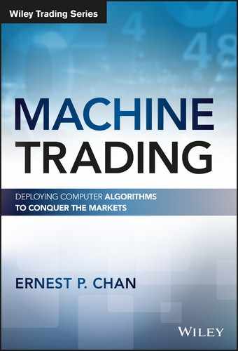
which comes back with a ADF test statistic of –3, while the critical value at 95 percent level is –2.9. So the ADF test also confirms that the BTC.USD price series is mean‐reverting and stationary. Hence a mean‐reversion trading strategy promises to be successful. But before we try that, let's just use AR(16) to predict the next price and buy or sell based on that prediction on the test set from September 3, 2014, to January 15, 2015. (This is the same strategy applied to AUD.USD in the Section on AR(p) in Chapter 3.) The CAGR is 40,000. The equity curve for the test set is shown in Figure 7.1.

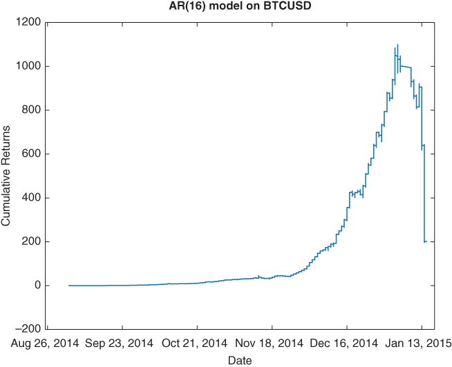
Image described by caption and surrounding text. — **Figure 7.1**: AR(16) trading strategy applied to BTC.USD

Is this return realistic? Of course not. One would need to assume that a limit order at midprice is always filled instantaneously to achieve this result. Nevertheless, it serves to illustrate that a simple AR(p) model has quite a bit of predictive power here.

We should also try ARMA(p, q) on BTC.USD. Following the same steps as we did for AUD.USD in the Section on ARMA(p, q) in Chapter 3, we find that the optimal p and q are $images$ and $images$ . We can then estimate the autoregressive and moving average coefficients on ARMA(3, 7) on BTC.USD, and use the resulting model to make one‐step‐ahead prediction as in the AR(16) case. Over the same test set, the CAGR is 3.9, which is still fantastic but much lower than the AR(16) model. The equity curve (Figure 7.2) also looks very different.

A plot of ARMA(3, 7) model on BTCUSD with Date on the horizontal axis, Cumulative Returns on the vertical axis, and a curve plotted. — **Figure 7.2**: ARMA(3, 7) trading strategy applied to BTC.USD

Mean Reversion Strategy

As we have ascertained via an AR(16) model as well as an ADF test in the previous section, the midprices of BTC.USD is a mean‐reverting, stationary, time series. This means a lot of simple mean‐reverting strategies described in Chan (2013) can be applied here.

The most well‐known mean reverting strategy is the Bollinger band strategy, where we buy a unit of BTC.USD when the midprice is $images$ moving standard deviations below the moving average, and sell when it is above. We will exit a position when the price mean reverts to the current moving average. This is illustrated in Figure 7.3. The moving standard deviation and average are on prices, not returns. The code fragment⁴ that generates the buy and sell signals is

buyEntry=cl  <= movingAvg(cl, lookback)-entryZscore*movingStd(cl, lookback);
sellEntry=cl >= movingAvg(cl, lookback)+entryZscore*movingStd(cl, lookback);

A diagram with our different curves labeled with arrows and different regions marked Upper band=MA+k*MSTD, Lower band=MA-k*MSTD, and Moving Average=MA. — **Figure 7.3**: Bollinger band trading strategy

Of course, we would stillneed to optimize the lookback as well as the multiple entryZscore. But we take the liberty of just arbitrarily deciding that the lookback should be 1 hour (60 bars for our minute‐bar data) and entryZscore should be 2. Running this on the same test set in the previous section (even though we didn't use the trainset for any training) yields a CAGR of 42 percent, with the equity curve displayed in Figure 7.4.

c07f004 — **Figure 7.4**: Bollinger band trading strategy on BTC.USD equity curve

Artificial Intelligence Techniques

Just like time series analysis, machine learning algorithms are another group of techniques that are helpful when we are faced with a market whose behavior is new to us, and we have not yet developed intuition about price patterns and arbitrage opportunities that may exist. So let's apply some of the algorithms we learned in Chapter 4 to the one‐minute bar BTC.USD data. To avoid learning spurious effects such as bid‐ask bounce, we will again use midprices for our analysis in this section throughout.

The first technique we will try is the regression algorithm with bagging. We merely copy the rTreeBagger.m program⁵ to apply to the data here. But instead of using ret1, ret2,…, ret20 as predictors, we use 1‐, 5‐, 10‐, 30‐, and 60‐minute bars returns. I will not display either the CAGR or the equity curve on the test set (which is the second half of the data set from January 20, 2014, to January 15, 2015), because they are simply too high to be realistic. This strategy clearly calls for a more careful backtest using bid‐ask quotes.

The second technique is the support vector machine. We can just copy the code svm.m from Chapter 4 ⁶ using the new predictors above. Lest you think that everything that worked with SPY will work even better with BTC.USD, here you will find quite negative returns for both train and test sets.

Finally, we will apply the feedforward neural network that we discussed in Chapter 4 as well.⁷ We will use a network with just one hidden layer and one neuron on that layer, but we will train 100 such networks with different initial guesses of the network parameters and average the predicted returns over all these networks. The out‐of‐sample return is as astounding as the one using the regression tree technique above, subject to the same caveats.

Order Flow

We discussed using order flow as an indicator for shortterm prediction in Chapter 6. Recall that order flow is signed transaction volume: if a transaction of size $images$ is the result of a buy market order, the order flow is $images$ ; if it is the result of a sell market order, the order flow is $images$ . Some bitcoin exchanges provide such data feeds with the “aggressor tag” that specifies whether a trade is the result of a buy or sell market order. This is the case with the BTC.CNY feed from BTC China and the BTC.USD feed from BitStamp. We will use a one‐month sample of the BTC.USD trade tick data from BitStamp to illustrate a trading strategy that uses order flow as a predictor. These data are time‐stamped to microseconds.

The trading strategy is in principle very simple. At the end of every microsecond bar, we look for all trade ticks within the past minute, and compute the order flow in that period. If this order flow is greater than some threshold, we send out a buy market order to buy a unit of BTC.USD, and vice versa for a sell market order. We will exit the resulting position, again using market orders, whenever the one‐minute order flow is zero or has the opposite sign from the one triggering the entry. The problem with this algorithm is that there are too many microsecond bars to loop through, and the program may need to run for a very long time. So we will instead backtest a simplified version of this strategy, using an event‐driven algorithm where we only compute order flow and decide whether to generate a trading signal when we encounter a trade tick. We also assume that our trade can be filled using this trade price, instead of using the current best bid or offer price. This is the same simplification we made in Example 6.3. The code details are discussed in Example 7.1. Naturally, both the entry threshold and the implicit exit threshold of zero, as well as the lookback period of one minute, should be optimized in‐sample and tested out‐of‐sample.

The backtest shows a profit of US$0.097 per one‐sided trade. With 336 such trades in December 2014, this translated to a profit of US$32.54 per coin, or an annualized return of approximately 100 percent. Of course, we should really be backtesting this high frequency strategy using bid‐ask quotes, as we have to execute this strategy by buying at the ask and selling at the bid. With a bid‐ask spread of about US$0.12, the transaction cost per trade is about US$0.06, which is still lower than the gross profit we computed. So there is hope that the strategy can generate a net profit, depending on the commissions that need to be paid. At the very least, this demonstrates that order flow is a reasonable predictor for bitcoin for this time frame.

Example 7.1: An order flow strategy

This example is similar to Example 6.3. It is very fortunate that we have access to the historical trades data from BitStamp that are time‐stamped at microseconds and more importantly, include the aggressor tag. This tag allows for accurate computation of order flow for our strategy. We save the aggressor tag in an array called $images$ , where $images$ indicates it is due to a buy market order, and $images$ indicates it is due to a sell market order. We will also save the trade size and price in arrays called $images$ and $images$ respectively, and compute the order flow as

ordflow=zeros(size(tradePrice));
ordflow(buy)=tradeSize(buy);
ordflow(sell)=-tradeSize(sell);

and the cumulative order flow as

cumOrdflow=smartcumsum(ordflow);

We will also keep track of the time stamp in an array dn, which contains the MATLAB datenum of the trades. All these arrays have the same dimension as the number of trade ticks. But note that trade ticks are not evenly spaced in time: There often are many consecutive microsecond bars that do not have any ticks and will not show up, and theoretically there can be multiple trades that share the same microsecond (though much less likely). If we go through these trades one‐by‐one, we can easily compute the net order flow within the last one minute:

for t=1:length(cumOrdflow)
    idx=find( dn  <= dn(t)-lookback/60/60/24);
    
    if (~isempty(idx))
        ordflow_lookback=cumOrdflow(t)-cumOrdflow(idx(end));
    end
end

The ordflow_lookback computed above can certainly be used to trigger a trade, whether for entry or exit. But even if time elapses without trades, the order flow within the last minute still needs to be updated. We are not actually doing that—we loop over only time bars that have trades, otherwise the program will take much longer to finish. What we are backtesting is really a slightly different version of the strategy described in the main text—one which is simpler to backtest. In this version, we only enter or exit when a trade occurs, therefore we only need to compute the order flow in the last minute at that time. For the original version, we will need to backtest with trades and quotes (TAQ) data, in addition to a more intelligent way to “fast forward” when there is no trade tick. (The backtest of this version will be left as an exercise.)

Continuing with our simplified strategy, we can insert the trade signal generator in the if‐block right after we compute ordflow_lookback:

if (ordflow_lookback > entryThreshold)
    if ( pos <= 0)
        if (pos < 0)
            dailyPL=dailyPL+(entryP-tradePrice(t));
            dailyNumTrade=dailyNumTrade+2;
            entryP=tradePrice(t);
        else
            entryP=tradePrice(t);
            dailyNumTrade=dailyNumTrade+1;
        end
        pos=1;
        
    end
elseif (ordflow_lookback < -entryThreshold)
    if (pos>= 0)
        if (pos > 0)
            dailyPL=dailyPL+(tradePrice(t)-entryP);
            dailyNumTrade=dailyNumTrade+2;
            entryP=tradePrice(t);
        else
            entryP=tradePrice(t);
            dailyNumTrade=dailyNumTrade+1;
        end
        pos=-1;
        
    end
else
    if (ordflow_lookback <= exitThreshold && pos > 0)
        dailyPL=dailyPL+(tradePrice(t)-entryP);
        dailyNumTrade=dailyNumTrade+1;
        pos=0;
    elseif (ordflow_lookback>= -exitThreshold && pos < 0)
        dailyPL=dailyPL+(entryP-tradePrice(t));
        dailyNumTrade=dailyNumTrade+1;
        pos=0;
    end
end

Before entering into the for‐loop, we should first initialize pos=0

pos=0;
dailyPL=0;
dailyNumTrade=0;

If we set entryThreshold to 90 and exitThreshold to 0, this simplified strategy generates a gross P&L of $32.54 for one unit of BTC.USD in December 2014, or $0.097 per one‐sided trade, assuming that we can get filled at the same trade price that triggered our trade. The complete code can be downloaded as orderFlow2.m.

Cross‐Exchange Arbitrage

Cross‐exchange arbitrage is only possible when the best bid price of an instrument on one exchange is higher than the best ask price of the same instrument on another exchange, so that we can buy at the market from the second exchange and then turn around and sell at the market on the first exchange, making a riskless profit.

There isn't much opportunity for cross‐exchange arbitrage in mature financial markets. Let's take the US stock market as an example. As we discussed in Chapter 6, though there are more than 60 exchanges or dark pools where one can trade AAPL, the “crossed market” situation described above will rarely occur due to Regulation NMS (“National Market System”) Rule 610 implemented by the SEC in 2005. Rule 610 requires an exchange to avoid displaying quotations that will cross the BBO quotes of another exchange (“Rule 610,” 2005). There goes our arbitrage opportunity!

There is still the possibility of engaging in cross‐border cross‐exchange arbitrage in stocks. For example, since IBM is traded in both NYSE and the LSE (London Stock Exchange), we may be able to spot the occasional crossed market situation after taking into account the exchange rate GBP.USD. But to make this trade really riskless, one has to hedge our currency risk. So, for example, if we bought some shares of IBM on LSE and sold equal number of shares of IBM in NYSE, we are essentially short GBP and long USD. We need to simultaneously buy some GBP.USD in order to hedge this currency exposure. This adds transaction costs and will reduce or eliminate our arbitrage profit.

In bitcoin markets, on the other hand, the opportunity for cross‐exchange arbitrage is seemingly abundant. Let's look at one example. At 7 p.m. EST on February 2, 2015, BTC.USD had the following bid‐ask quotes on two exchanges:

Bitfinex: 239.19–239.48
btc‐e: 233.232–233.546.

Why not sell a coin at $239.19 on Bitfinex, and immediately buy a coin at $233.546 on btc‐e, and earn a gross profit of US$5.644? In fact, the market is crossed like this for many days, even months. So why not do this continuously and becomes an overnight millionaire? To analyze whether there is really a free lunch to be had here, we have to look closely at the costs of the trade.

First, there is a commission of about 20 bps per side, which is about $1 for the complete transaction. Second, if we were to execute this continuously, we need to regularly withdraw a coin from btc‐e and transfer it to Bitfinex to cover our short position there. This withdrawal will cost about 1 percent, or $2. So we are left with about $2.6 net profit per coin—still excellent! But lastly, we have to be mindful why the quotes are lower at btc‐e. That is because the market judges it to have a lower credit rating. Since we have a long position there, we are exposed to credit risk.⁸ We have no easy method to compute whether this credit risk is higher or lower than the $2.6 per coin profit.

Summary

I have provided a whirlwind tour of some of the trading opportunities present in the bitcoin market. Bitcoin markets are still relatively immature compared to the stock or currency markets and, hence, there are still many inefficiencies and thus potentially profitable arbitrage opportunities. Some of these profits look outlandishly high—but are they real? That partly depends on your execution software's sophistication, the exchange's API efficiency, and its commissions and other fees, and finally, the creditworthiness of the exchange.

But beyond bitcoin, we also demonstrated how some of the techniques we developed in the previous chapters, such as time‐series analysis and artificial intelligence, can be brought to bear on an unfamiliar market. We also demonstrated the power of a universal short‐term indicator—order flow—and pointed out the mechanics of a cross‐border, cross‐exchange arbitrage that may be applicable to many more mature markets.

Exercises

7.1. Try the AR(p) and ARMA(p, q) models on BTC.USD on lower frequency time series such as 5‐minute, 15‐minute, and daily bars. Daily data can be downloaded from api.bitcoincharts.com/v1/csv/.
7.2. Backtest the strategy described in Example 7.1 where we may enter a trade even when there were no historical trades in a microsecond time bar. The best bid offer (BBO) data is available to download as 2014‐12_bbo.csv. Why must we backtest with BBO data in this case? Are there cases where we would enter into a new position with this strategy while our simplified version described in Example 7.1 would not? Is this version more or less profitable than the simplified version?

Endnotes

..................Content has been hidden....................

You can't read the all page of ebook, please click here login for view all page.

Table of Contents for Chapter 7: Bitcoins

Create new playlist

Sign In

Sign Up