
3
Some Recent Results on High Frequency Correlation
3.1 INTRODUCTION
In spite of its significant practical interest, high frequency correlation has not been widely studied in the literature. The main stylized fact known about it is the Epps effect [1979], which states that “correlations among price changes [...] are found to decrease with the length of the interval for which the price changes are measured”. Indeed, Figure 3.1 plots the correlation coefficient between the returns of the midquote of BNPP.PA and SOGN.PA, two major French financial stocks, as a function of the sampling period.
Figure 3.1 Correlation coefficient between the returns of the midquote of BNPP.PA and SOGN.PA as a function of the sampling period.
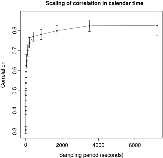
The correlation starts from a moderate value, 0.3, for a time scale of a few seconds, and then quickly reaches its asymptotic value, 0.8, after about 15 minutes of trading. Note that the increase in correlation between these two time scales is quite impressive since it is multiplied by more than 2.5. Note, however, that the correlation measured with daily closing prices during the same period is 0.94, still above the seemingly asymptotic value of the previous curve.
In this paper, we consider some empirical issues about high frequency correlation. First, we focus on how to extend the stochastic subordination framework introduced by Clark (1973) to the multivariate case. This allows us to model the random behavior of the covariance matrix of returns and the departure of the multivariate distribution of returns from the Gaussian. Then, we measure high frequency lead/lag relationships with the Hayashi–Yoshida (2005) cross-correlation estimator. Lead/lag is of high practical relevance because it can help to build statistical arbitrage strategies through its ability to forecast the short-term evolution of prices. Finally, we compute the intraday profile of correlation, which is also interesting for practitioners such as brokers who split the orders of their clients during the day. The intraday correlation impacts their trading schedule when dealing with a multi-asset portfolio.
The paper is organized as follows. Section 3.2 introduces the dataset. Section 3.3 elaborates on a generalization of event time to the multi-variate case. Then, Section 3.4 studies lead/lag relationships at high frequency. Section 3.5 gives some insight into the intraday profile of high frequency correlation. Finally, Section 3.6 concludes and announces further research.
3.2 DATA DESCRIPTION
We have access to the Reuters Tick Capture Engine (RTCE) database, which provides tick-by-tick data on many financial assets (equities, fixed income, forex, futures, commodities, etc.). Four levels of data are available:
- OHLC files: open, high, low, and close prices (on a given trading day);
- trades files: each transaction price and quantity timestamped up to the millisecond;
- quotes files: each quote (best bid and ask) price or quantity modification timestamped up to the millisecond;
- order book files: each limit price or quantity modification timestamped up to the millisecond, up to a given depth, typically ten limits on each side of the order book.
Throughout this study, we will use trades and quotes files. We will sample quotes on a trading time basis so that for each trade we have access to the quotes right before this trade. Trades and quotes data are recorded through different channels, which creates asynchrony between these two information sources. Therefore, a heuristic search algorithm is used to match trades and quotes.
When a trade walks the order book up or down by hitting consecutive limit prices, it is recorded as a sequence of trades with the same timestamp but with prices and quantities corresponding to each limit hit. For instance, assume that the best ask offers 100 shares at price 10 at 200 shares at price 10.01, and that a buy trade arrives for 150 shares. This is recorded as two lines in the trades file with the same timestamp, the first line being 100 shares at 10 and the second line 50 shares at 10.01. As a pre-processing step, we aggregate identical timestamps in the trades files by replacing the price by the volume weighted average price (VWAP) over the whole transaction and the volume by the sum of all quantities consumed. In the previous example, the trade price will thus be (100 × 10+50 × 10.01)/(100 + 50) = 10.00333 and the trade quantity is 100 + 50 = 150.
The assets we consider are mainly European stocks (except in Section 3.5) and also some major equity index futures. The futures are nearby-maturity futures and are rolled the day before the expiration date. We have data for these assets between 01/03/2010 and 31/05/2010. Except in Section 3.5, we drop the first and last hours of trading because they show a very diferent trading pattern from the rest of the day. By doing so, we limit seasonality effects. The returns we will consider are the returns of the midquote in order to get rid of the bid/ask bounce.
3.3 MULTIVARIATE EVENT TIME
3.3.1 Univariate case
Let us consider an asset whose price fluctuates randomly during the trading hours. Between the (i-1)th and the ith trade, the performance of the asset is simply ![]() . Then, N trades away from the opening price
. Then, N trades away from the opening price ![]() , the total variation is given by the product of these elementary ratios
, the total variation is given by the product of these elementary ratios

We are then left with the following expression for the relative price increment, i.e., the asset return
The asset return is clearly the sum of random variables and we would like to apply a version of the central limit theorem (CLT). The basic CLT is stated for independent and identically distributed random variables, a property that clearly fails to hold if one considers the returns of a financial asset: it has been well documented, and is easily verified experimentally, that absolute values of returns are autocorrelated (Bouchaud et al., 2004). However, the CLT can be extended to the more general case of weakly dependent variables ![]() (Whitt, 2002). The main condition for it to hold is the existence of the asymptotic variance
(Whitt, 2002). The main condition for it to hold is the existence of the asymptotic variance
assuming that the ![]() 's form a weak-sense stationary sequence.
's form a weak-sense stationary sequence.
If the sum above is finite, i.e. if the autocorrelation function of ![]() decays fast enough,1 then the CLT yields, as
decays fast enough,1 then the CLT yields, as ![]() ,
,
![]()
where ![]() and we have assumed2
and we have assumed2 ![]() . Hence, there holds, for
. Hence, there holds, for ![]() ,
,
![]()
i.e., returns are asymptotically normally distributed with variance proportional to the number of trades when they are sampled in trade time. Recast in the context of stochastic processes, the returns can therefore be viewed as a Brownian motion in a stochastic clock (such processes are called subordinated Brownian motions), the clock being the number of trades.
Note that the same line of reasoning can be used with the traded volume as the stochastic clock. Indeed, the return after a volume V has been traded is
where Vi is the volume traded during transaction i. NV is the number of transactions needed to reach an aggregated volume V. When scaling with the square root of the traded volume, we get
Since the volume of each transaction is finite, ![]() implies
implies ![]() . From the law of large numbers, we have
. From the law of large numbers, we have ![]() as
as ![]() , which is the average volume traded in a single transaction. Thus, applying Slutsky's theorem, we have, when
, which is the average volume traded in a single transaction. Thus, applying Slutsky's theorem, we have, when ![]() ,
,
![]()
Now, the number of trades or the traded volume over a time period is obviously random. Therefore, the ![]() -return
-return ![]() in calendar time exhibits a random variance
in calendar time exhibits a random variance ![]() , where
, where ![]() is either the number of trades or the traded volume occurring during a time period of length
is either the number of trades or the traded volume occurring during a time period of length ![]() . The distribution of calendar time returns
. The distribution of calendar time returns ![]() can be recovered from subordinated returns
can be recovered from subordinated returns ![]() through the application of Bayes' formula3
through the application of Bayes' formula3
![]()
where PZ(z) is the probability density function of the random variable Z. It is easy to show that the resulting distribution has fatter tails than the Gaussian (Abergel and Huth, in press). As mentioned in the introduction, this mechanism has been extensively studied in the finance literature (Silva, 2005), but only in the univariate framework. We want to generalize it to the multivariate case, which would turn into a stochastic covariance model to take into account the deviation of the empirical multivariate distribution of returns from the multivariate Gaussian.
3.3.2 Multivariate case
We now turn to the more interesting case of ![]() assets. How can we extend the previous framework to take several assets into account? Let us assume that an event time N is defined and that we sample returns
assets. How can we extend the previous framework to take several assets into account? Let us assume that an event time N is defined and that we sample returns ![]() according to this time. Using a multivariate CLT, we follow the same line of reasoning as in the previous section and obtain, for
according to this time. Using a multivariate CLT, we follow the same line of reasoning as in the previous section and obtain, for ![]() ,
,
![]()
where ![]() is now the covariance matrix.
is now the covariance matrix.
For a given time interval ![]() , the respective numbers of trades or traded volumes for each asset
, the respective numbers of trades or traded volumes for each asset ![]() are obviously different, and we need to define a global event time
are obviously different, and we need to define a global event time ![]() . We suggest to use
. We suggest to use ![]() , which amounts to increment time as soon as a trade occurs on any one of the d assets. This choice seems to us the simplest and most intuitive generalization of the univariate case, since it amounts to considering a single asset with dimension d: we aggregate the time series of the prices of each asset in chronological order, and then count trades or volumes as in the univariate case.4
, which amounts to increment time as soon as a trade occurs on any one of the d assets. This choice seems to us the simplest and most intuitive generalization of the univariate case, since it amounts to considering a single asset with dimension d: we aggregate the time series of the prices of each asset in chronological order, and then count trades or volumes as in the univariate case.4
3.3.3 Empirical results
In this section, we test our theory against high frequency multivariate data. The main statements are:
- Do returns become jointly normal when sampled in trade (respectively volume) time as N (respectively V) grows?
- Is the empirical covariance matrix of returns scaling linearly with N or V?
- What do
 and
and  look like?
We focus on four pairs of assets:
- BNPP.PA/SOGN.PA: BNP Paribas/Société Générale;
- RENA.PA/PEUP.PA: Renault/Peugeot;
- EDF.PA/GSZ.PA: EDF/GDF Suez;
- TOTF.PA/EAD.PA: Total/EADS.
Figure 3.2 QQ-plot of the squared Mahalanobis distance of returns sampled in volume time against chi-square quantiles with two degrees of freedom. The straight line depicts the 45∘ line. Top left panel: BNPP.PA/SOGN.PA. Top right panel: RENA.PA/PEUP.PA. Bottom left panel: EDF.PA/GSZ.PA. Bottom right panel: TOTF.PA/EAD.PA.
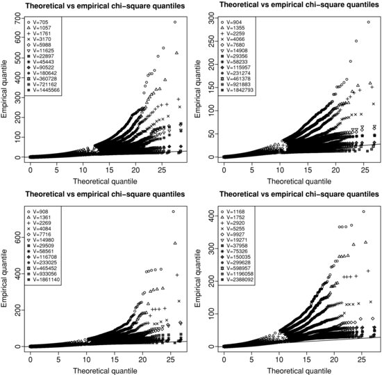
For sampling in trading time, we choose to sample every 2i trades for ![]() . The sampling in calendar and volume time are chosen so that they match the trading time sampling on average. This means that if we sample every N trades, then the corresponding time scale
. The sampling in calendar and volume time are chosen so that they match the trading time sampling on average. This means that if we sample every N trades, then the corresponding time scale ![]() is the average time that it takes to observe N consecutive trades. In the same way, V is the average volume traded after N trades. Since we want to avoid the use of overnight returns5 and to get approximately the same number of points for each sampling period, we sample prices with overlap. For instance, assume that we have a series of prices P1, P2, P3, P4, P5, and that we sample prices every two trades. Then we get three returns if we sample with overlap, namely (P3/P1), ln(P4/P2), ln(P5/P3). On the contrary, if we sample without overlap, we get two returns, ln(P3/P1), ln(P5/P3). The drawback of sampling with overlap is that points cannot be considered independent by construction.
is the average time that it takes to observe N consecutive trades. In the same way, V is the average volume traded after N trades. Since we want to avoid the use of overnight returns5 and to get approximately the same number of points for each sampling period, we sample prices with overlap. For instance, assume that we have a series of prices P1, P2, P3, P4, P5, and that we sample prices every two trades. Then we get three returns if we sample with overlap, namely (P3/P1), ln(P4/P2), ln(P5/P3). On the contrary, if we sample without overlap, we get two returns, ln(P3/P1), ln(P5/P3). The drawback of sampling with overlap is that points cannot be considered independent by construction.
Figure 3.2 displays the QQ-plot of the squared Mahalanobis distance of returns sampled in volume time against chi-square quantiles with two degrees of freedom for increasing sampling periods. The Mahalanobis distance of a random vector X is defined as ![]()
![]() , where
, where ![]() is its mean and Σ its covariance matrix. Standard computations show that if
is its mean and Σ its covariance matrix. Standard computations show that if ![]() , then D2 is distributed according to a chi-square with d degrees of freedom. Thus, for each observed bivariate return
, then D2 is distributed according to a chi-square with d degrees of freedom. Thus, for each observed bivariate return ![]() , we compute its Mahalanobis distance
, we compute its Mahalanobis distance ![]()
![]() , where μ and Σ are respectively the sample average and covariance matrix. We drop duplicates in the vector
, where μ and Σ are respectively the sample average and covariance matrix. We drop duplicates in the vector ![]() , which creates a new effective sample size n. We then plot the sorted
, which creates a new effective sample size n. We then plot the sorted ![]() against the chi-square quantiles
against the chi-square quantiles ![]() for i = 1, ..., n. Since n is of the order of 105 for our sample, we plot a point every 103 points and we keep every point in the last 103. If the empirical distribution agrees with the theoretical one, then points should lie on the 45° line. We see that the empirical Mahalanobis distances measured in volume time become closer to the chi-square distribution as the sampling period increases. This means that the probability of accepting the hypothesis of bivariate Gaussianity with success becomes larger with the event time scale. Note that for TOTF.PA/EAD.PA, returns sampled with the highest time scale under consideration (V = 2.38×10⁶) are a bit further from the straight line than other pairs. This might come from the difference of trading activity between these two stocks. The average duration between two trades for TOTF.PA is 3.283 seconds while it is 12.152 seconds for EAD.PA, which is 3.7 times longer. For BNPP.PA/SOGN.PA
(respectively RENA.PA/PEUP.PA, EDF.PA/GSZ.PA), this ratio is 1.01 (respectively 1.7, 1.5). Thus the bivariate event time might mostly be affected by TOTF.PA, leaving EAD.PA pretty much unchanged. As we mentioned before, the solution could be either to wait longer (measured in events) or to consider a new event time, such as the time it takes to have both assets updated at least a given number of times.
for i = 1, ..., n. Since n is of the order of 105 for our sample, we plot a point every 103 points and we keep every point in the last 103. If the empirical distribution agrees with the theoretical one, then points should lie on the 45° line. We see that the empirical Mahalanobis distances measured in volume time become closer to the chi-square distribution as the sampling period increases. This means that the probability of accepting the hypothesis of bivariate Gaussianity with success becomes larger with the event time scale. Note that for TOTF.PA/EAD.PA, returns sampled with the highest time scale under consideration (V = 2.38×10⁶) are a bit further from the straight line than other pairs. This might come from the difference of trading activity between these two stocks. The average duration between two trades for TOTF.PA is 3.283 seconds while it is 12.152 seconds for EAD.PA, which is 3.7 times longer. For BNPP.PA/SOGN.PA
(respectively RENA.PA/PEUP.PA, EDF.PA/GSZ.PA), this ratio is 1.01 (respectively 1.7, 1.5). Thus the bivariate event time might mostly be affected by TOTF.PA, leaving EAD.PA pretty much unchanged. As we mentioned before, the solution could be either to wait longer (measured in events) or to consider a new event time, such as the time it takes to have both assets updated at least a given number of times.
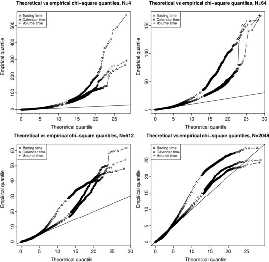
In comparison with volume time sampling, we plot on Figure 3.3 the same QQ-plot as on Figure 3.2, along with trading and calendar time sampling. We only show for visual clarity the results for the pair BNPP.PA/SOGN.PA and for four selected sampling periods. The findings are similar on the other pairs tested. From this figure it is clear that returns sampled in volume or trading time are closer to a bivariate Gaussian than calendar time returns, especially as the sampling period increases. Gaussianity seems even more plausible for volume time returns than for trading time returns.
Figure 3.3 QQ-plot of the squared Mahalanobis distance of returns sampled in trading, volume, and calendar time against chi-square quantiles with two degrees of freedom for BNPP.PA/SOGN.PA. Top left panel: N = 4. Top right panel: N = 64 . Bottom left panel: N = 512. Bottom right panel: N = 2048.
We now consider the scaling of the covariance matrix of returns in event time. Figure 3.4 (respectively 3.5) plots the realized variance (respectively covariance) of returns sampled in trading and volume time as a function of the sampling period, along with a linear fit. Clearly, the linearity of the covariance matrix as a function of either the volume or trading time is in agreement with the data. However, for very large sampling periods, the linearity tends to break down, but this might come from the shortage of data.
Figure 3.4 Scaling of the realized variance of returns sampled in volume (top panel) and trading (bottom panel) time as a function of the sampling period. The solid (respectively dotted) line shows the best linear fit with ordinary least squares on all points (respectively on all points except the last one). Left panel: BNPP.PA. Right panel: SOGN.PA.
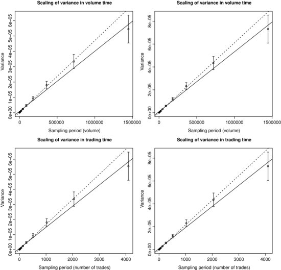
Figure 3.5 Scaling of the realized covariance of returns sampled in volume and trading time as a function of the sampling period for BNPP.PA/SOGN.PA. The solid (respectively dotted) line shows the best linear fit with ordinary least squares on all points (respectively on all points except the last one). Left panel: volume time. Right panel: trading time.
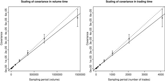
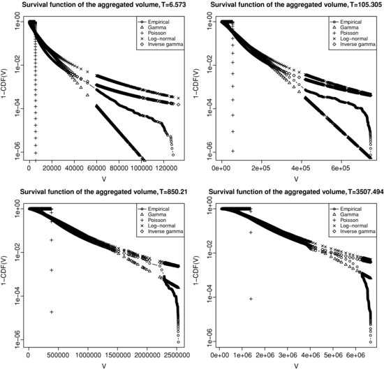
Figure 3.6 presents the survival function6 of the aggregated volume ![]() on a semi-log scale for four sampling periods
on a semi-log scale for four sampling periods ![]() . We consider four potential theoretical distributions as a comparison with the empirical one: Poisson, gamma, inverse-gamma and log-normal. We fit the parameters in order to match the first two moments of the empirical distribution. The empirical distribution lies somewhere in between the gamma distribution (exponential tail) and the inverse-gamma or log-normal distribution (heavy tails). Such a distribution for the subordinator respectively results in either a hyperbolic (exponential tails) or power-law (in the tails) distribution for price returns, which is in agreement with the deviation of the empirical distribution from the Gaussian.
. We consider four potential theoretical distributions as a comparison with the empirical one: Poisson, gamma, inverse-gamma and log-normal. We fit the parameters in order to match the first two moments of the empirical distribution. The empirical distribution lies somewhere in between the gamma distribution (exponential tail) and the inverse-gamma or log-normal distribution (heavy tails). Such a distribution for the subordinator respectively results in either a hyperbolic (exponential tails) or power-law (in the tails) distribution for price returns, which is in agreement with the deviation of the empirical distribution from the Gaussian.
Figure 3.6 Distribution of the aggregated volume ![]() for BNPP.PA/SOGN.PA and four sampling periods
for BNPP.PA/SOGN.PA and four sampling periods ![]() . Top left panel:
. Top left panel: ![]() = 6.573 seconds. Top right panel:
= 6.573 seconds. Top right panel: ![]() = 105.305 seconds. Bottom left panel:
= 105.305 seconds. Bottom left panel: ![]() = 850.21 seconds. Bottom right panel:
= 850.21 seconds. Bottom right panel: ![]() = 3507.494 seconds.
= 3507.494 seconds.
3.4 HIGH FREQUENCY LEAD/LAG
3.4.1 The Hayashi–Yoshida cross-correlation function
In Hayashi and Yoshida (2005), the authors introduce a new7 estimator of the linear correlation coefficient between two asynchronous diffusive processes. Given two Itô processes X, Y such that
and observation times ![]() for X and
for X and ![]() for Y, which must be independent from X and Y, they show that the following quantity
for Y, which must be independent from X and Y, they show that the following quantity
is an unbiased and consistent estimator of ![]() as the largest mesh size goes to zero, as opposed to the standard previous-tick covariance estimator (Griffin and Oomen, 2011; Zhang, 2011). In practice, it sums every product of increments as soon as they share any overlap of time. In the case of constant volatilities and correlation, it provides a consistent estimator for the correlation
as the largest mesh size goes to zero, as opposed to the standard previous-tick covariance estimator (Griffin and Oomen, 2011; Zhang, 2011). In practice, it sums every product of increments as soon as they share any overlap of time. In the case of constant volatilities and correlation, it provides a consistent estimator for the correlation
Recently, in Hoffman et al. (2010), the authors generalize this estimator to the whole cross-correlation function. They use a lagged version of the original estimator
It can be computed by shifting all the timestamps of Y and then using the Hayashi–Yoshida estimator. They define the lead/lag time as the lag that maximizes ![]() . In the following we will not estimate the lead/lag time but rather decide if one asset leads the other by measuring the asymmetry of the cross-correlation function between the positive and negative lags. More precisely, we state that X leads Y if X forecasts Y more accurately than Y does for X. Formally speaking, X is leading Y if
. In the following we will not estimate the lead/lag time but rather decide if one asset leads the other by measuring the asymmetry of the cross-correlation function between the positive and negative lags. More precisely, we state that X leads Y if X forecasts Y more accurately than Y does for X. Formally speaking, X is leading Y if
where Proj![]() denotes the projection of
denotes the projection of ![]() on the space spanned by
on the space spanned by ![]() . We will only consider the ordinary least squares setting, i.e. Proj
. We will only consider the ordinary least squares setting, i.e. Proj![]() and
and ![]() . In practice, we compute the cross-correlation function on a discrete grid of lags so that
. In practice, we compute the cross-correlation function on a discrete grid of lags so that ![]() . It is easy to show (see Appendix A) that
. It is easy to show (see Appendix A) that
![]() measures the correlation between Y and X. Indeed, X is a good predictor of Y if both are highly correlated. If we assume, furthermore, that the predictors X are uncorrelated, we can show that
measures the correlation between Y and X. Indeed, X is a good predictor of Y if both are highly correlated. If we assume, furthermore, that the predictors X are uncorrelated, we can show that
The asymmetry of the cross-correlation function, as defined by the LLR (standing for the lead/lag ratio) measures lead/lag relationships. Our indicator tells us which asset is leading the other for a given pair, but we might also wish to consider the strength and the characteristic time of this lead/lag relationship. Therefore, the maximum level of the cross-correlation function and the lag at which it occurs must also be taken into account.
In the following empirical study, we measure the cross-correlation function between variations of midquotes of two assets; i.e. X and Y are midquotes. The observation times will be tick times. Tick time is defined as the clock that increments each time there is a nonzero variation of the midquote between two trades (not necessarily consecutive). It does not take into account the nil variations of the midquote, contrary to trading time.
3.4.2 Empirical results
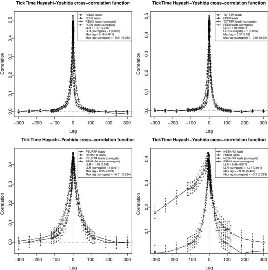
Figure 3.7 shows the tick time Hayashi–Yoshida cross-correlation functions computed on four pairs of assets:
- FCE/FSMI: future/future;
- FCE/TOTF.PA: future/stock;
- RENA.PA/PEUP.PA: stock/stock;
- FSMI/NESN.VX: future/stock.
Figure 3.7 Tick time Hayashi–Yoshida cross-correlation function. Top left panel: FCE/FSMI. Top right panel: FCE/TOTF.PA. Bottom left panel: RENA.PA/PEUP.PA. Bottom right panel: FSMI/NESN.VX.
We choose the following grid of lags (in seconds):
![]()
We consider that there is no correlation after five minutes of trading on these assets, which seems to be empirically justified on Figure 3.7, except for the FSMI/NESN.VX case. Figure 3.8 is similar to Figure 3.7, but zooms on lags smaller than 10 seconds. In order to assess the robustness of our empirical results against the null hypothesis of no genuine lead/lag relationship but only artificial lead/lag, we build a surrogate dataset. For two assets and for a given trading day, we generate two synchronously correlated Brownian motions with the same correlation as the two assets ![]() on [0, T], T being the duration of a trading day, with a mesh of 0.01 second. Then we sample these Brownian motions along the true timestamps of the two assets, so that the surrogate data have the same timestamp structure as the original data. The error bars indicate the 95 % confidence interval for the average correlation over all trading days.8
on [0, T], T being the duration of a trading day, with a mesh of 0.01 second. Then we sample these Brownian motions along the true timestamps of the two assets, so that the surrogate data have the same timestamp structure as the original data. The error bars indicate the 95 % confidence interval for the average correlation over all trading days.8
Figure 3.8 Zoom on lags smaller than 10 seconds in Figure 3.7.
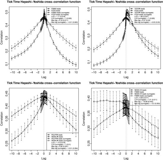
For the FCE/FSMI pair (future versus future), the cross-correlation vanishes very quickly and there is less than 5 % of correlation at 30 seconds. We observe that there is more weight on the side where FCE leads with an LLR of 1.17 and a maximum correlation at 0.16 seconds. The pair FCE/TOTF.PA involves a future on an index with a stock being part of this index. Not surprisingly, the future leads by 0.37 seconds. This pair shows the biggest amount of lead/lag as measured by the LLR (1.85). The RENA.PA/PEUP.PA case compares two stocks in the French automobile industry. The cross-correlation is the most symmetric of the four shown with an LLR of 1.15. Finally, the FSMI/NESN.VX pair is interesting because the stock leads the future on the index where it belongs. Indeed, this result might be explained by the fact that NESN.VX is the largest market capitalization in the SMI, about 25 %. The asymmetry is quite strong (LLR = 0.69) and the maximum lag is 16.89 seconds, which is very large, but there is a significant amount of noise on this average lag. We also see that there still seems to be correlation after five minutes. The difference between the maximum correlation and the correlation at lag zero is 4.5 % for FCE/FSMI, 4.7 % for FCE/TOTF.PA, 1.4 % for RENA.PA/PEUP.PA, and 2.4 % for FSMI/NESN.VX, which confirms that the lead/lag is less pronounced for RENA.PA/PEUP.PA. The LLR for surrogate data is equal to one and the maximum lag is very close to zero for the four pairs of assets.9 This strong contrast between real and surrogate data suggests that there are genuine lead/lag relationships between these assets that are not solely due to the difference in the levels of trading activity.
A more detailled study of lead/lag relationships, and especially their link with liquidity, will be available in Abergel and Huth (forthcoming 2012b).
3.5 INTRADAY SEASONALITY OF CORRELATION
Trading activity on financial markets is well known to display intraday seasonality (Abergel et al., 2011a; Admati and Pfleiderer, 1988; Andersen and Bollerslev, 1997; Chan et al., 1995). Seasonality appears on many quantities of interest, such as volatility, transaction volume, bid/ask spread, market and limit orders arrivals, etc. For instance, the intraday pattern of the traded volume on European equity stocks obeys an asymmetric U-shape: big volumes at the opening of the market, then it decreases until lunch time where it reaches the minimum, after 13:3010 it starts to rise again, peaks at 14:30 (announcement of macroeconomic figures), it changes regime at 15:30 (NYSE and NASDAQ openings), peaks at 16:00 (other macroeconomic figures), and finally rallies to reach its highest level at the close of the market. Therefore, the intraday seasonality seems to be highly connected with both the human activity and the arrival of significant information. We believe that huge volumes at the opening are due to the discovery of both corporate news and figures (earnings, dividends, etc.) before the market opens, the information coming from other international market performances and the adjustment of positions taken the day before, while the peak at the close is made by large investors such as derivatives traders and portfolio managers who benchmark on closing prices.
In order to compute the intraday profile of correlation, or any other quantity of interest, we cut trading days into 5 minute bins spanning the whole day from the open to the close of the market. For instance, on the CAC40 universe, the market opens at 9:00 and closes at 17:30, which leads to 8.5 × 12 = 102 bins. On each day, we compute statistics on each time slice and then we average over days for each slice. We end up with an average statistics for each 5 minute bin. More precisely, for a given bin b = 1, ..., B, the resulting statistics is
where Sd(b) is the statistics computed on day d and bin b. In order to compare the results from one universe to the other, we normalize the intraday profile by the average value of the profile
![]()
Since we have data for many stocks, we display cross-sectional results; i.e., we compute a statistics independently on each asset (or pair of assets if we are interested in bivariate statistics) and we typically plot the probability distribution of this statistics over the universe.
We focus our study on four universes of stocks:
- the 40 assets composing the French index CAC40 on 01/03/2010 (CAC universe);
- the 30 most liquid11 assets from the English index Footsie100 on 01/03/2010 (FTSE universe);
- the 30 assets comprising the US index DJIA on 01/03/2010, plus major financial and IT stocks, 40 US stocks altogether (NY universe);
- the 30 assets composing the Asian index TopixCore30 on 01/03/2010 (TOPIX universe).
We use the Hayashi–Yoshida (2005) estimator for covariance and the standard realized volatility estimator (Barndorff-Nielsen and Shephard, 2002). We consider midquotes sampled in trading time, i.e. ![]() (resp.
(resp. ![]() ) is the midquote of asset X (resp. Y) just before the trade that occurred at time ti (resp. sj) on X (resp. Y).
) is the midquote of asset X (resp. Y) just before the trade that occurred at time ti (resp. sj) on X (resp. Y).
3.5.1 Empirical results
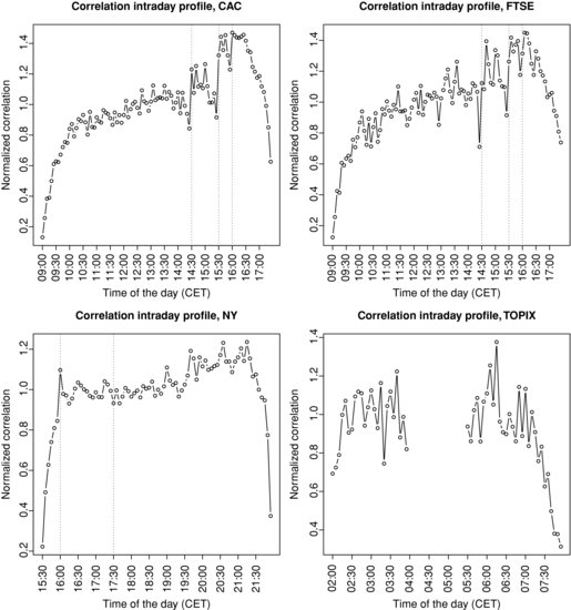
Figure 3.9 plots the intraday profile of correlation for the four universes and Figure 3.10 zooms on cross-sectional medians of profiles normalized by their average.12 The CAC and FTSE correlation profiles are very similar and show an upward trend. The correlation is substantially weak at the open and steadily increases until 14:00; then there is a sudden strong upward jump at 14:30 when most of the US macroeconomic figures are announced.13 At 15:30 (NYSE and NASDAQ markets open), we observe another sharp jump in correlation, followed by another jump at 16:00 when other macroeconomic figures are known by market participants. After 16:00, correlation tends to decrease to roughly 60 % (respectively 70 %) of its daily average at the close for the CAC (respectively FTSE) universe. Another remarkable pattern in this profile is that there is always a downard trend starting 15 or 20 minutes before abrupt jumps.
Figure 3.9 Intraday profile of correlation (cross-sectional distribution). Top left panel: CAC universe. Top right panel: FTSE universe. Bottom left panel: NY universe. Bottom right panel: TOPIX universe.
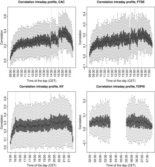
Figure 3.10 Intraday profile of normalized correlation (cross-sectional median). Top left panel: CAC universe. Top right panel: FTSE universe. Bottom left panel: NY universe. Bottom right panel: TOPIX universe.
Regarding the NY universe, the correlation is also very low at the open and increases up to 16:00, where the aforementioned jump related to US figures occurs. We do not observe a significant impact when European stock markets close (17:30), in contrast to the noteworthy impact of US markets opening on Europe. The upward trend continues until 21:15, after which the correlation drops to reach 40 % of its average daily level. Most of this massive decrease in correlation is realized during the last 10 minutes of the trading session.
The intraday profile for the TOPIX universe is cut into two pieces because of the trading halt on the Tokyo Stock Exchange between 03:00 and 04:30. Both trading sessions tend to be similar to the patterns already observed on other universes: a global upward trend with a drop at the close. Note that the gap between the correlation at the first close and at the second open is quite small, roughly 10 % of the average daily level.
Finally, we remark that the TOPIX cross-sectional distribution of correlation is the tightest and smallest, with an average correlation of about 5 % and many negatively correlated stocks, while the three other universes exhibit about 25 % of the average correlation, with not very much negative correlation.
The modeling of this intraday correlation pattern with nonstationary Hawkes processes will be studied in Abergel and Huth (forthcoming 2012a).
3.6 CONCLUSION
This paper provides some recent empirical results on high frequency correlation. We introduce a generalization of the univariate event time to take into account several assets. The resulting model for the distribution of returns fits the data quite well. We observe significant lead/lag relationships at high frequency, especially in the future/stock case. Finally, we study the intraday pattern of correlation and find a seemingly universal pattern, where correlation starts from small values and increases throughout the day, but substantially drops one hour before the closing of the market.
Regarding further research, lead/lag relationships will be investigated in more detail in Abergel and Huth (forthcoming 2012b), and we also plan to use the branching structure of Hawkes processes (Ogata et al., 2002) to estimate the distribution of the lead/lag time. A forthcoming paper by Abergel and Huth (2012a) will be devoted to the calibration of the intraday correlation pattern with nonstationary Hawkes processes using the EM algorithm introduced in Lewis and Mohler (2011).
ACKNOWLEDGMENT
The authors would like to thank the members of the Natixis statistical arbitrage R&D team for fruitful discussions.
REFERENCES
Abergel, F. and N. Huth (forthcoming 2012a) High Frequency Correlation Intraday Profile. Empirical Facts.
Abergel, F. and N. Huth (forthcoming 2012b) High Frequency Lead/Lag Relationships. Empirical Facts.
Abergel, F. and N. Huth (in press). The Times Change: Multivariate Subordination. Empirical Facts, to appear in Quantitative Finance.
Abergel, F., A. Chakraborti, I. Muni Toke and M. Patriarca (2011a) Econophysics Review: 1. Empirical Facts, Quantitative Finance 11(7), 991–1012.
Abergel, F., A. Chakraborti, I. Muni Toke and M. Patriarca (2011b) Econophysics Review: 2. Agent-Based Models, Quantitative Finance 11(7), 1013–1041.
Admati, A. and P. Pfleiderer (1988) A Theory of Intraday Patterns: Volume and Price Variability, Review of Financial Studies 1(1), 3–40.
Andersen, T. and T. Bollerslev (1997) Intraday Periodicity and Volatility Persistence in Financial Markets, Journal of Empirical Finance 4, 115–158
Barndorff-Nielsen, O. and N. Shephard (2002) Econometric Analysis of Realized Volatility and Its Use in Estimating Stochastic Volatility Models, Journal of the Royal Statistical Society, Series B (Statistical Methodology) 64(2), 253–280.
Bouchaud, J.-P., Y. Gefen, M. Potters and M. Wyart (2004) Fluctuations and Response in Financial Markets: The Subtle Nature of ``Random'' Price Changes, Quantitative Finance 4(2), 176–190.
Chan, K., Y.P. Chung and H. Johnson (1995) The Intraday Behavior of Bid-Ask Spreads for NYSE Stocks and CBOE Options, Journal of Financial and Quantitative Analysis 30(3), 329–346.
Clark, P.K. (1973) A Subordinated Stochastic Process Model with Finite Variance for Speculative Prices, Econometrica 41, 135–155.
De Jong, F. and T. Nijman (1997) High Frequency Analysis of Lead–Lag Relationships between Financial Markets, Journal of Empirical Finance 4(2–3), 259–277.
Epps, T.W. (1979) Comovements in Stock Prices in the Very Short-Run, Journal of the American Statistical Association 74, 291–298.
Griffin, J.E. and R.C.A. Oomen (2011) Covariance Measurement in the Presence of Non-Synchronous Trading and Market Microstructure Noise, Journal of Econometrics 160(1), 58–68.
Hayashi, T. and N. Yoshida (2005) On Covariance Estimation of Non-Synchronously Observed Diffusion Processes, Bernoulli 11(2), 359–379.
Hoffmann, M., M. Rosenbaum and N. Yoshida (2010) Estimation of the Lead–Lag Parameter From Nonsynchronous Data, to Appear in Bernoulli.
Lewis, E. and G. Mohler (2011) A Nonparametric EM algorithm for Multiscale Hawkes Processes, Working Paper.
Ogata, Y., D. Vere-Jones and J. Zhuang (2002) Stochastic Declustering of Space–Time Earthquake Occurrences, Journal of the American Statistical Association 97, 369–380.
Silva, A.C. (2005) Applications of Physics to Finance and Economics: Returns, Trading Activity and Income. PhD Thesis.
Whitt, W. (2002) Stochastic-Process Limits, Springer.
Zhang, L. (2011) Estimating Covariation: Epps Effect, Microstructure Noise, Journal of Econometrics 160(1), 33–47.
1. In the case of price returns ![]() , the autocorrelation function decays very fast and can be considered as statistically insignificant after some lag k close to one, even for small time scales (Abergel et al., 2011a). Therefore the above sum is finite in practice.
, the autocorrelation function decays very fast and can be considered as statistically insignificant after some lag k close to one, even for small time scales (Abergel et al., 2011a). Therefore the above sum is finite in practice.
2. It is a reasonable assumption since we are dealing with high frequency data.
3. We assume that the distribution of the trading activity ![]() (number of trades or traded volume) can be approximated by a continuous distribution.
(number of trades or traded volume) can be approximated by a continuous distribution.
4. Such a representation makes sense when the orders of magnitude of the liquidity of each of the d assets are similar: consider the extreme case of one heavily traded asset and another one with only one trade per day. In this case, the normality of the couple as ![]() increases may fail to appear before an unrealistically large number of trades. A more appropriate clock might thus be to wait until each asset has been updated at least N times, which amounts to choosing
increases may fail to appear before an unrealistically large number of trades. A more appropriate clock might thus be to wait until each asset has been updated at least N times, which amounts to choosing ![]() .
.
5. The use of overnight returns would be inappropriate in our framework because there is a significant trading activity during the opening and closing auctions, which would bias the event time clocks. Moreover, we want to focus only on the intraday behavior of returns when there is continuous trading between the starting and ending timestamps of returns.
6. The survival function of a random variable X is defined as S(x) = P(X > x).
7. In fact, a very similar estimator was already designed by De Jong and Nijman (1997).
8. Assuming our dataset is made of D uncorrelated trading days, the confidence interval for the average correlation ![]() , where
, where ![]() . By doing so, we neglect the variance of the correlation estimator inside a day.
. By doing so, we neglect the variance of the correlation estimator inside a day.
9. In fact, it can be assumed to be zero with a confidence level of 95%.
10. In the following, we will always use Central European Time.
11. We use here the average daily number of trades as a rough criterion of liquidity.
12. The whisker plots we present display a box ranging from the first to the third quartile with the median in between and whiskers extending to the most extreme point that is no more than 1.5 times the interquartile range from the box. These are the default settings in the boxplot function of R.
13. The figures released at 14:30 are the Consumer Price Index, the Durable Goods Report, the Employee Cost Index, the Existing Home Sales, the Factory Orders Report, the Gross Domestic Product, the Housing Starts, the Jobless Claims Report, the Personal Income and Outlays, the Producer Price Index, the Productivity Report, the Retail Sales Report, and the Trade Balance Report. Those released at 16:00 are the Consumer Confidence Index, the Non-Manufacturing Report, the Purchasing Managers Index, and the Wholesale Trade Report. All of these figures are released on a monthly basis, except the GDP, which is announced quarterly.