
5
Models for the Impact of All Order Book Events
5.1 INTRODUCTION
The relation between order flow and price changes has attracted considerable attention in recent years (see Hasbrouck, 2007; Mike and Farmer, 2008; Bouchaud et al., 2004, 2006, 2009; Lyons, 2006). Most empirical studies to date have focused on the impact of (buy/sell) market orders. Many interesting results have been obtained, such as the very weak dependence of impact on the volume of the market order, the long-range nature of the sign of the trades, and the resulting nonpermanent, power-law decay of market order impact with time (see Bouchaud et al., 2009). However, this representation of impact is incomplete in at least two ways. First, the impact of all market orders is usually treated on the same footing, or with a weak dependence on volume, whereas some market orders are “aggressive” and immediately change the price, while others are more passive and only have a delayed impact on the price. Second, other types of order book events (limit orders, cancellations) must also directly impact prices: adding a buy limit order induces extra upwards pressure and cancelling a buy limit order decreases this pressure. Within a description based on market orders only, the impact of limit orders and cancellations is included in an indirect way, in fact as an effectively decaying impact of market orders. This decay reflects the “liquidity refill” mechanism explained in detail by Bouchaud et al. (2006, 2009), Weber and Rosenow (2005), Gerig (2008), and Farmer et al. (2006), whereby market orders trigger a counterbalancing flow of limit orders.
A framework allowing one to analyze the impact of all order book events and to understand in detail the statistical properties of price time series is clearly desirable. Surprisingly, however, there are only very few quantitative studies of the impact of limit orders and cancellations (Hautsch and Huang, 2009; Eisler et al., 2011) – partly due to the fact that more detailed data, beyond trades and quotes, is often needed to conduct such studies. The aim of the present paper is to provide a theoretical framework for the impact of all order book events, which allows one to build statistical models with intuitive and transparent interpretations (Eisler et al., 2011).
5.2 A SHORT SUMMARY OF MARKET ORDER IMPACT MODELS
A simple model relating prices to trades posits that the mid-point price pt just before trade t can be written as a linear superposition of the impact of all past trades (Bouchaud et al., 2004, 2006):
where vt is the volume of the trade at time t, ![]() the sign of that trade (+ for a buy, − for a sell), and
the sign of that trade (+ for a buy, − for a sell), and ![]() is an independent noise term that models any price change not induced by trades (e.g., jumps due to news). The exponent
is an independent noise term that models any price change not induced by trades (e.g., jumps due to news). The exponent ![]() is found to be small. The most important object in the above equation is the function
is found to be small. The most important object in the above equation is the function ![]() describing the temporal evolution of the impact of a single trade, which can be called a “propagator”: how does the impact of the trade at time
describing the temporal evolution of the impact of a single trade, which can be called a “propagator”: how does the impact of the trade at time ![]() propagate, on average, up to time t? Because the signs of trades are strongly autocorrelated,
propagate, on average, up to time t? Because the signs of trades are strongly autocorrelated, ![]() must decay with time in a very specific way, in order to maintain the (statistical) efficiency of prices. Clearly, if
must decay with time in a very specific way, in order to maintain the (statistical) efficiency of prices. Clearly, if ![]() did not decay at all, the returns1 rt=pt+1−pt would simply be proportional to the sign of the trades, and therefore would themselves be strongly autocorrelated in time. The resulting price dynamics would then be highly predictable, which is not realistic. The result of Bouchaud et al. (2004) is that if the correlation of signs
did not decay at all, the returns1 rt=pt+1−pt would simply be proportional to the sign of the trades, and therefore would themselves be strongly autocorrelated in time. The resulting price dynamics would then be highly predictable, which is not realistic. The result of Bouchaud et al. (2004) is that if the correlation of signs ![]() decays at large
decays at large ![]() as
as ![]() with
with ![]() (as found empirically), then
(as found empirically), then ![]() must decay as
must decay as ![]() with
with ![]() for the price to be exactly diffusive at long times. The impact of single trades is therefore predicted to decay as a power-law (at least up to a certain time scale).
for the price to be exactly diffusive at long times. The impact of single trades is therefore predicted to decay as a power-law (at least up to a certain time scale).
The above model can be rewritten in a completely equivalent way in terms of returns, with a slightly different interpretation (Gerig, 2008; Farmer et al., 2006):
This can be read as saying that the tth trade has a permanent impact on the price, but this impact is history dependent and depends on the sequence of past trades. The fact that G decays with ![]() implies that the kernel
implies that the kernel ![]() is negative, and therefore that a past sequence of buy trades (
is negative, and therefore that a past sequence of buy trades (![]() ) tends to reduce the impact of a further buy trade but increase the impact of a sell trade. This is again a consequence of the dynamic nature of liquidity: when trades persist in a given direction, opposing limit orders tend to pile up and reduce the average impact of the next trade in the same direction. For the price to be an exact martingale, the quantity
) tends to reduce the impact of a further buy trade but increase the impact of a sell trade. This is again a consequence of the dynamic nature of liquidity: when trades persist in a given direction, opposing limit orders tend to pile up and reduce the average impact of the next trade in the same direction. For the price to be an exact martingale, the quantity ![]() must be equal to the conditional expectation of
must be equal to the conditional expectation of ![]() at time t−, such that
at time t−, such that ![]() is the surprise part of
is the surprise part of ![]() . This condition allows one to recover the above mentioned decay of
. This condition allows one to recover the above mentioned decay of ![]() at large
at large ![]() .
.
In order to calibrate the model, one can use the empirically observable impact function ![]() , defined as
, defined as
(5.3) ![]()
and the time correlation function ![]() of the variable
of the variable ![]() to map out, numerically, the complete shape of
to map out, numerically, the complete shape of ![]() . This was done by Bouchaud et al. (2006), using the exact relation
. This was done by Bouchaud et al. (2006), using the exact relation
Alternatively, one can use the “return” version of the model, Equation (5.2), which gives
(5.5) ![]()
which in turn leads to
As noted in Sérié (2010), this second implementation is in fact much less sensitive to finite size effects and therefore more adapted to data analysis.2
The above model, regardless of the type of fitting, is approximate and incomplete in two interrelated ways. First, Equations (5.1) and (5.2) neglect the fluctuations of the impact: one expects in general that G and ![]() should depend both on t and t' and not only on
should depend both on t and t' and not only on ![]() . Impact can indeed be quite different depending on the state of the order book and the market conditions at t'. As a consequence, if one blindly uses Equations (5.1) and (5.2) to compute the second moment of the price difference,
. Impact can indeed be quite different depending on the state of the order book and the market conditions at t'. As a consequence, if one blindly uses Equations (5.1) and (5.2) to compute the second moment of the price difference, ![]() , with a nonfluctuating
, with a nonfluctuating ![]() calibrated to reproduce the impact function
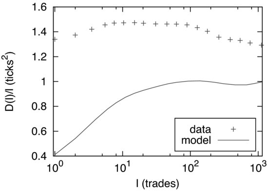
calibrated to reproduce the impact function ![]() , the result clearly underestimates the empirical price variance (see Figure 5.1).
, the result clearly underestimates the empirical price variance (see Figure 5.1).
Figure 5.1 ![]() and its approximation with the transient impact model (TIM) with only trades as events, with
and its approximation with the transient impact model (TIM) with only trades as events, with ![]() and for small tick stocks. Results are shown when assuming that all trades have the same, nonfluctuating impact
and for small tick stocks. Results are shown when assuming that all trades have the same, nonfluctuating impact ![]() , calibrated to reproduce
, calibrated to reproduce ![]() . This simple model accounts for
. This simple model accounts for ![]() of the long-term volatility. Other events and/or the fluctuations of
of the long-term volatility. Other events and/or the fluctuations of ![]() must therefore contribute to the market volatility as well.
must therefore contribute to the market volatility as well.
Adding a diffusive noise ![]() would only shift
would only shift ![]() upwards, but this is insufficient to reproduce the empirical data. Second, as noted in the introduction, other events of the order book can also change the mid-price, such as limit orders placed inside the bid-ask spread, or cancellations of all the volume at the bid or the ask. These events do indeed contribute to the price volatility and should be explicitly included in the description. A simplified description of price changes in terms of market orders only attempts to describe other events of the order book in an effective way, through the nontrivial time dependence of
upwards, but this is insufficient to reproduce the empirical data. Second, as noted in the introduction, other events of the order book can also change the mid-price, such as limit orders placed inside the bid-ask spread, or cancellations of all the volume at the bid or the ask. These events do indeed contribute to the price volatility and should be explicitly included in the description. A simplified description of price changes in terms of market orders only attempts to describe other events of the order book in an effective way, through the nontrivial time dependence of ![]() .
.
In the following, we will generalize the above model to account for the impact of other types of events, beyond market orders. In this case, however, it will become apparent that the two versions of the above model are no longer equivalent, and lead to different quantitative results. Our main objective will be to come up with a simple, intuitive model that (i) can be easily calibrated on data, (ii) reproduces as closely as possible the second moment of the price difference ![]() , (iii) can be generalized to richer and richer data sets, where more and more events are observable, and (iv) can in principle be systematically improved.
, (iii) can be generalized to richer and richer data sets, where more and more events are observable, and (iv) can in principle be systematically improved.
5.3 MANY-EVENT IMPACT MODELS
5.3.1 Notation and definitions
The dynamics of the order book is rich and complex, and involves the intertwined arrival of many types of events. These events can be categorized in different, more or less natural types. In the empirical analysis presented below, we have considered the following six types of events:
- market orders that do not change the best price (noted MO0) or that do change the price (noted MO'),
- limit orders at the current bid or ask (LO0) or inside the bid-ask spread so that they change the price (LO'), and
- cancellations at the bid or ask that do not remove all the volume quoted there (CA0) or that do (CA').
Of course, events deeper in the order book could also be added, as well as any extra division of the above types into subtypes, if more information is available. For example, if the identity code of each order is available, one can classify each event according to its origin, as was done in Tóth et al. (2011). The generic notation for an event type occurring at event time t will be ![]() . The upper index ′ (“prime”) will denote that the event changed any of the best prices, and the upper index 0 that it did not. Abbreviations without the upper index (MO, CA, LO) refer to both the price changing and the price non-changing event type. Every event is given a sign
. The upper index ′ (“prime”) will denote that the event changed any of the best prices, and the upper index 0 that it did not. Abbreviations without the upper index (MO, CA, LO) refer to both the price changing and the price non-changing event type. Every event is given a sign ![]() according to its expected long-term effect on the price – the precise definitions are summarized in Table 5.1. Note that the table also defines the gaps
according to its expected long-term effect on the price – the precise definitions are summarized in Table 5.1. Note that the table also defines the gaps ![]() , which will be used later. We will rely on indicator variables denoted as
, which will be used later. We will rely on indicator variables denoted as ![]() . This expression is equal to 1 if the event at t is of type
. This expression is equal to 1 if the event at t is of type ![]() and zero otherwise. We also use the notation
and zero otherwise. We also use the notation ![]() to denote the time average of the quantity between the brackets.
to denote the time average of the quantity between the brackets.
Table 5.1 Summary of the six possible event types and the corresponding definitions of the event signs and gaps
Let us now define the response of the price to different types of orders. The average behavior of price after events of a particular type ![]() defines the corresponding response function (or the average impact function):
defines the corresponding response function (or the average impact function):
Where the right-hand side of the bracket indicates a conditional average over t's where πt = π. This is equivalent to a correlation function between ![]() at time t and the price change from t to
at time t and the price change from t to ![]() , normalized by the stationary probability of the event
, normalized by the stationary probability of the event ![]() , denoted as
, denoted as ![]() . This normalized response function gives the expected directional price change after an event
. This normalized response function gives the expected directional price change after an event ![]() . Its behavior for all
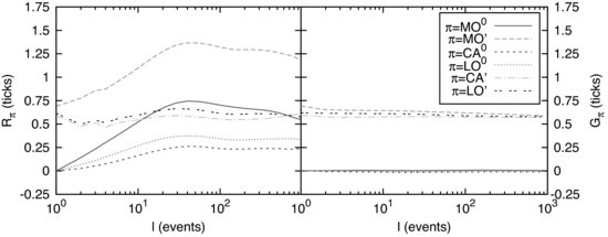
. Its behavior for all ![]() 's is shown on the left of Figure 5.2. Tautologically,
's is shown on the left of Figure 5.2. Tautologically, ![]() for price changing events and
for price changing events and ![]() for the others. Empirically, all types of events lead, on average, to a price change in the expected direction, i.e.,
for the others. Empirically, all types of events lead, on average, to a price change in the expected direction, i.e., ![]() .
.
Figure 5.2 (left) The response function ![]() and (right) the bare impact function
and (right) the bare impact function ![]() for the TIM, for the data described in Section 5.4.1. The curves are labeled according to
for the TIM, for the data described in Section 5.4.1. The curves are labeled according to ![]() in the legend. Note that
in the legend. Note that ![]() is to a first approximation independent of
is to a first approximation independent of ![]() for all
for all ![]() 's. However, the small variations are real and important to reproduce the correct price diffusion curve
's. However, the small variations are real and important to reproduce the correct price diffusion curve ![]() .
.
We will also need the “return” response function, upgrading the quantity ![]() defined above to a matrix:
defined above to a matrix:
(5.8) ![]()
Clearly, as an exact identity,
(5.9) ![]()
Similarly, the signed-event correlation function is defined as
(5.10) ![]()
Our convention is that the first index corresponds to the first event in chronological order. Note that, in general, there are no reasons to expect time reversal symmetry, which would impose ![]() . If one has N event types, altogether there are N2 of these event–event correlations and return response functions.
. If one has N event types, altogether there are N2 of these event–event correlations and return response functions.
5.3.2 The transient impact model (TIM)
Let us write down the natural generalization of the above transient impact model (TIM), embodied by Equation (5.1), to the many-event case. We now envisage that each event type ![]() has a “bare” time dependent impact given by
has a “bare” time dependent impact given by ![]() , such that the price reads
, such that the price reads
where one selects, for each t', the propagator ![]() corresponding to the particular event type at that time. After straightforward calculations, the response function (5.7) can be expressed as
corresponding to the particular event type at that time. After straightforward calculations, the response function (5.7) can be expressed as
This is a direct extension of Equation (5.4). One can invert the system of Equations (5.12) to evaluate the unobservable ![]() 's in terms of the observable
's in terms of the observable ![]() 's and
's and ![]() 's – see Figure 5.2 (right). Note that we formulate the problem here in terms of the “derivatives” of the
's – see Figure 5.2 (right). Note that we formulate the problem here in terms of the “derivatives” of the ![]() 's since, as mentioned above, it is numerically much more stable to introduce new variables for the increments of
's since, as mentioned above, it is numerically much more stable to introduce new variables for the increments of ![]() and G and solve (5.12) in terms of those.
and G and solve (5.12) in terms of those.
Once this is known, one can explicitly compute the lag dependent diffusion constant ![]() in terms of the G's and the C's, generalizing the corresponding result obtained by Bouchaud et al. (2004) (see the Appendix).
in terms of the G's and the C's, generalizing the corresponding result obtained by Bouchaud et al. (2004) (see the Appendix).
5.3.3 The history dependent impact model (HDIM)
Now, if one wants to generalize the history dependent impact model (HDIM), Equation (5.2), to the many-event case, one immediately realizes that the impact at time t depends on the type of event one is considering. For one thing, the instantaneous impact of price nonchanging events is trivially zero. For price changing events, ![]() , the instantaneous impact is given by
, the instantaneous impact is given by
Here ![]() depends on the type of price changing event
depends on the type of price changing event ![]() that happens then, and possibly also on the sign of that event. For example, if
that happens then, and possibly also on the sign of that event. For example, if ![]() and
and ![]() this means that a sell market order executed the total volume at the bid. The mid-quote price change is
this means that a sell market order executed the total volume at the bid. The mid-quote price change is ![]() , which usually means that the second best level was at
, which usually means that the second best level was at ![]() , where bt is the bid price before the event. The factor 2 is necessary, because the ask did not change, and the impact is defined by the change of the mid-quote. Hence
, where bt is the bid price before the event. The factor 2 is necessary, because the ask did not change, and the impact is defined by the change of the mid-quote. Hence ![]() 's for MO''s (and similarly CA''s) correspond to half of the gap between the first and the second best quote just before the level was removed (see also Farmer et al., 2004). Another example is when
's for MO''s (and similarly CA''s) correspond to half of the gap between the first and the second best quote just before the level was removed (see also Farmer et al., 2004). Another example is when ![]() and
and ![]() . This means that at t a sell limit order was placed inside the spread. The mid-quote price change is
. This means that at t a sell limit order was placed inside the spread. The mid-quote price change is ![]() , which means that the limit order was placed at
, which means that the limit order was placed at ![]() , where at is the ask price. Thus
, where at is the ask price. Thus ![]() for LO''s correspond to half of the gap between the first and the second best quote right after the limit order was placed. In the following we will call the
for LO''s correspond to half of the gap between the first and the second best quote right after the limit order was placed. In the following we will call the ![]() 's gaps. For large tick stocks, these nonzero
's gaps. For large tick stocks, these nonzero ![]() 's are most of the time equal to half a tick, and only very weakly fluctuating. For small tick stocks, substantial fluctuations of the spread and of the gaps behind the best quotes can take place. The generalization of Equation (5.2) precisely attempts to capture these gap fluctuations, which are affected by the flow of past events. If we assume that the whole dynamical process is statistically invariant under exchanging buy orders with sell orders (
's are most of the time equal to half a tick, and only very weakly fluctuating. For small tick stocks, substantial fluctuations of the spread and of the gaps behind the best quotes can take place. The generalization of Equation (5.2) precisely attempts to capture these gap fluctuations, which are affected by the flow of past events. If we assume that the whole dynamical process is statistically invariant under exchanging buy orders with sell orders (![]() ) and bids with asks, the dependence on the current nonzero gaps on the past order flow can only include an even number of
) and bids with asks, the dependence on the current nonzero gaps on the past order flow can only include an even number of ![]() 's. Therefore the lowest order model for nonzero gaps (including a constant term and a term quadratic in
's. Therefore the lowest order model for nonzero gaps (including a constant term and a term quadratic in ![]() 's) is
's) is
where ![]() are kernels that model the dependence of the gaps on the past order flow (note that
are kernels that model the dependence of the gaps on the past order flow (note that ![]() is a
is a ![]() matrix) and
matrix) and ![]() are the average realized gaps, defined as
are the average realized gaps, defined as ![]() , since the average of the second term in the right-hand side is identically zero. Note that the last term, equal to
, since the average of the second term in the right-hand side is identically zero. Note that the last term, equal to ![]() , was not explicitly included in our previous analysis (Eisler et al., 2011). However, typical values are less than 1 % of the average realized gap, and therefore negligible in practice. We set it to zero in the following.
, was not explicitly included in our previous analysis (Eisler et al., 2011). However, typical values are less than 1 % of the average realized gap, and therefore negligible in practice. We set it to zero in the following.
Equation (5.14), combined with the definition of the return at time t, Equation (5.13), leads to our generalization of the HDIM, Equation (5.2):
It is interesting to compare the above equation with its analog for the transient impact model, which reads (after Equation (5.11))
(5.16) ![]()
The two models can only be equivalent if
which means that the “influence matrix” ![]() has a much constrained structure, which has no reason to be optimal. It is also a priori inconsistent since the TIM leads to a nonzero price move even if
has a much constrained structure, which has no reason to be optimal. It is also a priori inconsistent since the TIM leads to a nonzero price move even if ![]() is a price nonchanging event, since Equation (5.17) is valid for all event types
is a price nonchanging event, since Equation (5.17) is valid for all event types ![]() . This is a major conceptual drawback of the TIM framework (although, as we will see below, the model fares quite well at reproducing the price diffusion curve).
. This is a major conceptual drawback of the TIM framework (although, as we will see below, the model fares quite well at reproducing the price diffusion curve).
The matrix ![]() can in principle be determined from the empirical knowledge of the response matrices
can in principle be determined from the empirical knowledge of the response matrices ![]() , since
, since
(5.18) 
Note, however, that the last term includes a three-body correlation function that is not very convenient to estimate. At this stage and below, we need to make some approximation to estimate higher order correlations. We assume that all three- and four-body correlation functions can be factorized in terms of two-body correlation functions, as if the variables were Gaussian. This allows us to extract ![]() from a numerically convenient expression, used in Eisler et al. (2011):
from a numerically convenient expression, used in Eisler et al. (2011):
Knowing the ![]() 's and using the same factorization approximation, one can finally estimate the price diffusion constant, given in the Appendix. Although the factorization approximation used to obtain the diffusion constant looks somewhat arbitrary, we find that it is extremely precise when applied to the diffusion curve.
's and using the same factorization approximation, one can finally estimate the price diffusion constant, given in the Appendix. Although the factorization approximation used to obtain the diffusion constant looks somewhat arbitrary, we find that it is extremely precise when applied to the diffusion curve.
For large tick stocks, the gaps hardly vary with time and are all equal to one tick. In other words, ![]() and the model simplifies enormously, since now
and the model simplifies enormously, since now ![]() . In this limit, one therefore finds
. In this limit, one therefore finds
which means that the total price response to some event can be understood as its own impact (lag zero), plus the sum of the biases in the course of future events, conditional to this initial event. These biases are multiplied by the average price change ![]() that these induced future events cause. Within the same model, the volatility reads
that these induced future events cause. Within the same model, the volatility reads
For small ticks, on the other hand, gaps do fluctuate and react to the past order flow; the influence matrix ![]() describes how the past order flow affects the current gaps. If
describes how the past order flow affects the current gaps. If ![]() is positive, it means that an event of type
is positive, it means that an event of type ![]() (price changing or not) tends to increase the gaps (i.e. reduce the liquidity) for a later price changing event
(price changing or not) tends to increase the gaps (i.e. reduce the liquidity) for a later price changing event ![]() in the same direction and decrease the gap if the sign of the event
in the same direction and decrease the gap if the sign of the event ![]() is opposite to that of
is opposite to that of ![]() .
.
5.4 MODEL CALIBRATION AND EMPIRICAL TESTS
5.4.1 Data
We have tested the above ideas on a set of data made of 14 randomly selected liquid stocks traded on the NASDAQ during the period 03/03/2008 to 19/05/2008, a total of 53 trading days (see Eisler et al., 2011, for a detailed presentation of these stocks and summary statistics). In order to reduce the effects of the intraday spread and liquidity variations we exclude the first 30 and the last 40 minutes of the trading days. The particular choice of market is not very important; many of our results were also verified on other markets, such as CME Futures, US Treasury Bonds, and stocks traded at the London Stock Exchange.
Our sample of stocks can be divided into two groups: large tick and small tick stocks. Large tick stocks are such that the bid-ask spread is almost always equal to one tick, whereas small tick stocks have spreads that are typically a few ticks. The behavior of the two groups is quite different; for example, the events that change the best price have a relatively low probability for large tick stocks (about 3 % altogether), but not for small tick stocks (up to 40 %). Note that there is a number of stocks with intermediate tick sizes, which to some extent possess the characteristics of both groups. Technically, they can be treated in exactly the same way as small tick stocks, and all our results remain valid. However, for the clarity of presentation, we will not consider them explicitly.
As explained above, we restrict ourselves to events that modify the bid or ask price, or the volume quoted at these prices. Events deeper in the order book are unobserved and will not be described: although they do not have an immediate effect on the best quotes, our description is still incomplete. Furthermore, we note that the stocks we are dealing with are traded on multiple platforms. This may account for some of the residual discrepancies reported below.
Since we consider six types of events, there are six response functions ![]() and propagators
and propagators ![]() , and 36 correlation functions
, and 36 correlation functions ![]() . However, since the return response functions
. However, since the return response functions ![]() and the influence kernels
and the influence kernels ![]() are nonzero only when the second event
are nonzero only when the second event ![]() is a price changing event, there are only
is a price changing event, there are only ![]() of them.
of them.
5.4.2 The case of large ticks
As explained in the previous section, the case of large ticks is quite simple since the gap fluctuation term of HDIM can be neglected altogether. As shown in Eisler et al. (2011), the predictions given by Equations (5.20) and (5.21) are in very good agreement with the empirical determination of the ![]() and the price diffusion
and the price diffusion ![]() . Small remaining discrepancies can indeed be accounted for by adding the gap fluctuation contribution, of the order of a few percent.
. Small remaining discrepancies can indeed be accounted for by adding the gap fluctuation contribution, of the order of a few percent.
The temporary impact model, on the other hand, is not well adapted to describe large tick stocks, for the following reason: when Equation (5.12) is used to extract ![]() from the data, small numerical errors may lead to some spurious time dependence. However, as far as
from the data, small numerical errors may lead to some spurious time dependence. However, as far as ![]() is concerned, any small variation of
is concerned, any small variation of ![]() is amplified through the second term of Equation (5.24) in the Appendix, which is an infinite sum of positive terms. As noted in Eisler et al. (2011), this leads to large discrepancies between the predicted
is amplified through the second term of Equation (5.24) in the Appendix, which is an infinite sum of positive terms. As noted in Eisler et al. (2011), this leads to large discrepancies between the predicted ![]() and its empirical determination. At any rate, one should clearly favor the calibration of
and its empirical determination. At any rate, one should clearly favor the calibration of ![]() using Equation (5.12) rather than the analog of Equation (5.4).
using Equation (5.12) rather than the analog of Equation (5.4).
5.4.3 The case of small ticks
The case of small ticks is much more interesting, since in this case the role of gap fluctuations is crucial and is a priori a stringent test for the two models on stage.
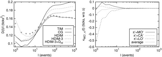
Figure 5.3 (left) ![]() and its approximations. Crosses correspond to the data. The constant gap (CG) model corresponds to
and its approximations. Crosses correspond to the data. The constant gap (CG) model corresponds to ![]() . TIM corresponds to the temporary impact model calibrated on returns. The curve for HDIM uses the approximate calibration of
. TIM corresponds to the temporary impact model calibrated on returns. The curve for HDIM uses the approximate calibration of ![]() 's, where HDIM-3 is taking 3 times the
's, where HDIM-3 is taking 3 times the ![]() 's as from the calibration. We also indicate HDIM-3 by adding the constant Dhf=0.04. Note that the vertical scale is different from Figure 5.1, since the time clock is different in the two cases (all events versus trades in Figure 5.1). (right) Comparison of the three nonzero
's as from the calibration. We also indicate HDIM-3 by adding the constant Dhf=0.04. Note that the vertical scale is different from Figure 5.1, since the time clock is different in the two cases (all events versus trades in Figure 5.1). (right) Comparison of the three nonzero ![]() with their average over
with their average over ![]() . Note that
. Note that ![]() : after an MO' event, gaps on the same side are on average smaller.
: after an MO' event, gaps on the same side are on average smaller.
5.4.3.1 TIM
Within the temporary impact model, the response functions ![]() are tautologically accounted for, since they are used to calibrate the propagators
are tautologically accounted for, since they are used to calibrate the propagators ![]() using Equation (5.12). Once the
using Equation (5.12). Once the ![]() 's are known (see Figure 5.2, where
's are known (see Figure 5.2, where ![]() and
and ![]() are shown for small tick stocks), one can compute the time dependent diffusion coefficient
are shown for small tick stocks), one can compute the time dependent diffusion coefficient ![]() and compare it with empirical data. This is shown in Figure 5.3 (left). Note that we calibrate the
and compare it with empirical data. This is shown in Figure 5.3 (left). Note that we calibrate the ![]() for each stock separately, compute
for each stock separately, compute ![]() in each case, and then average the results over all stocks. The agreement is surprisingly good for long times, while for shorter times the model underestimates price fluctuations, which is expected since the model does not allow for high frequency fluctuations. We also show the prediction based on the constant gap approximation,
in each case, and then average the results over all stocks. The agreement is surprisingly good for long times, while for shorter times the model underestimates price fluctuations, which is expected since the model does not allow for high frequency fluctuations. We also show the prediction based on the constant gap approximation, ![]() . Although Figure 5.2 suggests that this is an acceptable assumption, we see that
. Although Figure 5.2 suggests that this is an acceptable assumption, we see that ![]() is overestimated. As will be argued below, gaps do adapt to past order flow, and the net effect of the gap dynamics is to reduce the price volatility. We finally note that calibrating the
is overestimated. As will be argued below, gaps do adapt to past order flow, and the net effect of the gap dynamics is to reduce the price volatility. We finally note that calibrating the ![]() on the response functions directly (and not on their derivatives), as was done in Eisler et al. (2011), leads to much poorer results for the diffusion coefficient
on the response functions directly (and not on their derivatives), as was done in Eisler et al. (2011), leads to much poorer results for the diffusion coefficient ![]() .
.
5.4.3.2 HDIM
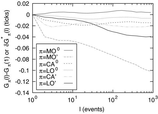
We now turn to the history dependent impact model. As explained above, we determine the influence kernels ![]() using Equation (5.19). We plot in Figure 5.4 the resulting “integrated impact” on the future gaps of all six
using Equation (5.19). We plot in Figure 5.4 the resulting “integrated impact” on the future gaps of all six ![]() events, which we define as3
events, which we define as3
(5.22) ![]()
As explained in Eisler et al. (2011), ![]() captures the contribution of the gap “compressibility” to the impact of an event of type
captures the contribution of the gap “compressibility” to the impact of an event of type ![]() up to a time lag
up to a time lag ![]() , leaving the sequence of events unchanged. If
, leaving the sequence of events unchanged. If ![]() were independent of
were independent of ![]() , as postulated in the TIM, one would have
, as postulated in the TIM, one would have ![]() as an identity. The agreement turns out to be excellent (see Figure 5.4), which was not guaranteed a priori since the HDIM is calibrated on a much larger set of correlation functions.
as an identity. The agreement turns out to be excellent (see Figure 5.4), which was not guaranteed a priori since the HDIM is calibrated on a much larger set of correlation functions.
Figure 5.4 The integrated impact on the future gaps ![]() in the HDIM estimated via Equation (5.17). The results are indistinguishable from
in the HDIM estimated via Equation (5.17). The results are indistinguishable from ![]() calculated for the TIM. The curves are labeled according to
calculated for the TIM. The curves are labeled according to ![]() in the legend.
in the legend.
However, this does not mean that ![]() 's are necessarily independent of
's are necessarily independent of ![]() . To illustrate the point that Equation (5.17) is too restrictive, Figure 5.3 (right) compares the three
. To illustrate the point that Equation (5.17) is too restrictive, Figure 5.3 (right) compares the three ![]() 's, which are clearly different from one another. Note that the average over
's, which are clearly different from one another. Note that the average over ![]() is negative, meaning that MO' events tend to “harden” the book (i.e. after an MO' event, gaps on the same side are on average smaller). This is true for all price changing events, while (perhaps surprisingly) small market orders MO0 “soften” the book:
is negative, meaning that MO' events tend to “harden” the book (i.e. after an MO' event, gaps on the same side are on average smaller). This is true for all price changing events, while (perhaps surprisingly) small market orders MO0 “soften” the book: ![]() is positive and gaps tend to grow. Queue fluctuations (CA0 and LO0) seem less important, but for small ticks these types of events also harden the book. Note finally that for large ticks
is positive and gaps tend to grow. Queue fluctuations (CA0 and LO0) seem less important, but for small ticks these types of events also harden the book. Note finally that for large ticks ![]() 's are found to be about two orders of magnitude smaller, which confirms that gap fluctuations can be neglected in that case.
's are found to be about two orders of magnitude smaller, which confirms that gap fluctuations can be neglected in that case.
Now, Equation (5.19) relies on the factorization of a three-point correlation function and is not exact, so there is no guarantee that the response functions ![]() are exactly reproduced using this calibration method. In order to check this approximation, we have simulated an artificial market dynamics where the price evolves according to Equation (5.15), with the true (historical) sequence of signs and events and
are exactly reproduced using this calibration method. In order to check this approximation, we have simulated an artificial market dynamics where the price evolves according to Equation (5.15), with the true (historical) sequence of signs and events and ![]() . The kernels
. The kernels ![]() are calibrated using Equation (5.19). This leads to the predictions shown as dashed lines in Figure 5.5. The agreement can be much improved by simply multiplying all
are calibrated using Equation (5.19). This leads to the predictions shown as dashed lines in Figure 5.5. The agreement can be much improved by simply multiplying all ![]() 's by a factor 3 (see Figure 5.5). Of course, some discrepancies remain and one should use the historical simulation systematically to determine the optimal
's by a factor 3 (see Figure 5.5). Of course, some discrepancies remain and one should use the historical simulation systematically to determine the optimal ![]() 's. This is, however, numerically much more difficult and an improved analytical approximation of the three-point correlation function, which would allow a more accurate workable calibration, would be welcome.
's. This is, however, numerically much more difficult and an improved analytical approximation of the three-point correlation function, which would allow a more accurate workable calibration, would be welcome.
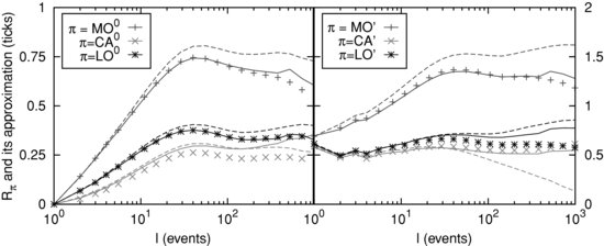
Figure 5.5 ![]() and their approximation with the HDIM. Symbols correspond to data: they are perfectly in line with the model prediction under the assumption that approximation (5.19) is correct. The dashed lines correspond to the response function of an actual simulation of the model with the
and their approximation with the HDIM. Symbols correspond to data: they are perfectly in line with the model prediction under the assumption that approximation (5.19) is correct. The dashed lines correspond to the response function of an actual simulation of the model with the ![]() 's calibrated via Equation (5.19). The solid lines correspond to the simulation if we increase all calibrated
's calibrated via Equation (5.19). The solid lines correspond to the simulation if we increase all calibrated ![]() 's by a factor 3 (HDIM-3). The lines vary according to
's by a factor 3 (HDIM-3). The lines vary according to ![]() , as shown in the legend.
, as shown in the legend.
Finally, we computed ![]() for the HDIM using (5.25) in the Appendix. Here again, we have tested the quality of the factorization approximation using the same historical simulation. In this case, the
for the HDIM using (5.25) in the Appendix. Here again, we have tested the quality of the factorization approximation using the same historical simulation. In this case, the ![]() curve is indistinguishable from its approximation, so any discrepancy between the data and formula (5.25) cannot be blamed on its approximate nature, but rather on an inadequate calibration of the
curve is indistinguishable from its approximation, so any discrepancy between the data and formula (5.25) cannot be blamed on its approximate nature, but rather on an inadequate calibration of the ![]() 's.
's.
The result is given in Figure 5.3 (left) together with the previous theoretical predictions and the empirical data.4 With the naïve calibration the HDIM turns out to be worse than the TIM for large lags: it overestimates ![]() by 15 % or so. Increasing the
by 15 % or so. Increasing the ![]() 's by a factor of 3 again greatly improves the fit but part of the discrepancy remains. For small lags, one needs to add a constant contribution
's by a factor of 3 again greatly improves the fit but part of the discrepancy remains. For small lags, one needs to add a constant contribution ![]() to match the data.5 The HDIM produces a significant improvement over the constant gap model, because it explicitly includes the effect of gap fluctuations. However, since the calibration procedure relies on an approximation, we do not reproduce the response functions exactly. Hence the better founded model (HDIM) fares worse in practice than a model with theoretical inconsistencies (TIM). As noted above, a better calibration procedure for the
to match the data.5 The HDIM produces a significant improvement over the constant gap model, because it explicitly includes the effect of gap fluctuations. However, since the calibration procedure relies on an approximation, we do not reproduce the response functions exactly. Hence the better founded model (HDIM) fares worse in practice than a model with theoretical inconsistencies (TIM). As noted above, a better calibration procedure for the ![]() 's could improve the situation.
's could improve the situation.
At any rate, numerical discrepancies should be expected regardless of the fitting procedure, since we have neglected several effects, which must be present. These include (i) all volume dependence, (ii) unobserved events deeper in the book and on other platforms, and (iii) higher order, nonlinear contributions to model history dependence. On the last point, we note that based on symmetry arguments, the gap fluctuation term may include higher order terms of the form
(5.23) ![]()
or with a larger (even) number of ![]() 's. The presence of a four
's. The presence of a four ![]() term is in fact suggested by the data shown in Figure 13 of Eisler et al. (2011), and also by more recent analysis (Tóth, 2011). It would be interesting to study these effects in detail, and understand their impact on price diffusion.
term is in fact suggested by the data shown in Figure 13 of Eisler et al. (2011), and also by more recent analysis (Tóth, 2011). It would be interesting to study these effects in detail, and understand their impact on price diffusion.
5.5 CONCLUSION
Let us summarize what we have tried to accomplish in the present paper. Our aim was to provide a general framework to describe the impact of different events in the order book, in a way that is flexible enough to deal with any classification of these events (provided this classification makes sense).6 We have specifically considered market orders, limit orders, and cancellation at the best quotes, further subdividing each category into price changing and price nonchanging events, giving a total of six types. In trying to generalize previous work, which focused on the impact of market orders only, we have discovered that two different models can be envisaged. These are equivalent when only a single event type, market orders regardless of their aggressivity, are taken into account. One model posits that each event type has a temporary impact (TIM), whereas the other assumes that only price changing events have a direct impact, which is itself modulated by the past history of all events, a model we called “history dependent impact” (HDIM).
The TIM is a natural extension of Hasbrouck's VAR model to a multi-event setting: one writes a vector autoregression model for the return at time t in terms of all signed past events, but neglects the direct influence of past returns themselves (although these would be easy to include if needed). We have discussed the fact that TIMs are, strictly speaking, inconsistent since they assign a nonzero immediate impact to price nonchanging events. Still, provided the model is correctly calibrated using returns (see Equation (5.12)), we find that the TIM framework allows one to reproduce the price diffusion pattern surprisingly accurately.
The HDIM family can also be thought of as a VAR model, although one now distinguishes between different types of event-induced returns before regressing them on past events. The HDIM is interesting because it gives a very appealing interpretation of the price changing process in terms of history dependent “gaps”, which determine the amplitude of the price jump if a certain type of price changing event takes place. We have in particular defined a lag dependent, ![]() “influence matrix” (called
“influence matrix” (called ![]() in the text), which tells us how much, on average, an event of type
in the text), which tells us how much, on average, an event of type ![]() affects the immediate impact of a
affects the immediate impact of a ![]() price changing event of the same sign in the future.
price changing event of the same sign in the future.
The HDIM therefore envisages the dynamics of prices as consisting of three processes: instantaneous jumps due to events, events inducing further events and thereby affecting the future jump probabilities (described by the correlation between events), and events exerting pressure on the gaps behind the best price and thereby affecting the future jump sizes (described by the ![]() 's). By describing this third effect with a linear regression process, we came up with the explicit model (5.15), which can be calibrated on empirical data provided some factorization approximation is made (which unfortunately turns out not to be very accurate, calling for further work on this matter). This allows one to measure the influence matrix
's). By describing this third effect with a linear regression process, we came up with the explicit model (5.15), which can be calibrated on empirical data provided some factorization approximation is made (which unfortunately turns out not to be very accurate, calling for further work on this matter). This allows one to measure the influence matrix ![]() and its lag dependence. We find in particular that price changing events, such as aggressive market orders MO', tend to reduce the impact of later events of the same sign (i.e. a buy MO' following a buy MO') but increase the impact of later events of the opposite sign. As stressed in Bouchaud et al. (2009), Gerig (2008), and Farmer et al. (2006), this history dependent asymmetric liquidity is the dominant effect that mitigates persistent trends in prices that would otherwise be induced by the long-ranged correlation in the sign of market orders.
and its lag dependence. We find in particular that price changing events, such as aggressive market orders MO', tend to reduce the impact of later events of the same sign (i.e. a buy MO' following a buy MO') but increase the impact of later events of the opposite sign. As stressed in Bouchaud et al. (2009), Gerig (2008), and Farmer et al. (2006), this history dependent asymmetric liquidity is the dominant effect that mitigates persistent trends in prices that would otherwise be induced by the long-ranged correlation in the sign of market orders.
In spite of these enticing features, we have found that the HDIM leads to a worse determination of the price diffusion properties than the TIM. The almost perfect agreement between the TIM prediction and empirical data is perhaps accidental, but it may also be that TIMs (which have fewer parameters) are numerically more robust than HDIMs. For HDIMs, a more accurate calibration procedure is needed. This could be achieved either by finding a better, workable approximation for the three-point correlation function or by using a purely numerical approach based on a historical simulation of the HDIM. On the other hand, some effects have been explicitly neglected, such as the role of unobserved events deeper in the book and on other platforms, or possible nonlinearities in the history dependence of gaps. It would be very interesting to investigate the relevance of these effects and to come up either with a fully consistent version of HDIM or with a convincing argument for why the TIM appears to be particularly successful.
In any case, we hope that the intuitive and versatile framework that we proposed above, together with operational calibration procedures, will help to make sense of the highly complex and intertwined sequences of events that take place in the order books, and allows one to build a comprehensive theory of price formation in electronic markets.
APPENDIX
Expression of the price diffusion for the TIM and HDIM
We give here the rather ugly looking explicit expressions for the diffusion curve ![]() in both models. For the TIM, one gets as an exact expression:
in both models. For the TIM, one gets as an exact expression:
where D0 is the variance of the noise term ![]() .
.
For the HDIM, on the other hand, one has to use a factorization approximation to compute three- and four-point correlation functions in terms of two-point correlations. One can finally estimate the price diffusion constant, which is given by the following approximate equation (Eisler et al., 2011):
where D0 is again the variance of the noise ![]() ,
,
(5.26) 
and, for ![]() ,
,
(5.27) 
whereas for t<0, we use ![]() . We also introduced a correlation function between event types as (Eisler et al., 2011):
. We also introduced a correlation function between event types as (Eisler et al., 2011):
(5.28) 
ACKNOWLEDGMENTS
The authors are grateful to Emmanuel Sérié for his ideas on fitting impact kernels. They also thank Bence Tóth for his critical reading and comments.
REFERENCES
Bouchaud, J.-P., Y. Gefen, M. Potters and M. Wyart (2004) Fluctuations and Response in Financial Markets: The Subtle Nature of “Random” Price Changes, Quantitative Finance 4, 176.
Bouchaud, J.-P., J.D. Farmer and F. Lillo (2009) How Markets Slowly Digest Changes in Supply and Demand, in Handbook of Financial Markets: Dynamics and Evolution, T. Hens and K.R. Schenk-Hoppe (Eds), North-Holland, Elsevier.
Bouchaud, J.-P., J. Kockelkoren and M. Potters (2006) Random Walks, Liquidity Molasses and Critical Response in Financial Markets, Quantitative Finance 6, 115.
Eisler, Z., J.-P. Bouchaud and J. Kockelkoren (2011) The Price Impact of Order Book Events: Market Orders, Limit Orders and Cancellations, arXiv:0904.0900, to appear in Quantitative Finance.
Farmer, J.D., L. Gillemot, F. Lillo, S. Mike and A. Sen (2004) What Really Causes Large Price Changes? Quantitative Finance 4, 383.
Farmer, J.D., A. Gerig, F. Lillo and S. Mike (2006) Market Efficiency and the Long-Memory of Supply and Demand: Is Price Impact Variable and Permanent or Fixed and Temporary?, Quantitative Finance 6, 107.
Gerig, A. (2008) A Theory for Market Impact: How Order Flow Affects Stock Price, PhD Thesis, arXiv:0804.3818.
Hasbrouck, J. (2007) Empirical Market Microstructure: The Institutions, Economics, and Econometrics of Securities Trading, Oxford University Press.
Hautsch, N. and R. Huang (2009) The Market Impact of a Limit Order, Working Paper.
Lyons, R.K. (2006) The Microstructure Approach to Exchange Rates, MIT Press.
Mike, S. and J.D. Farmer (2008) An Empirical Behavioral Model of Liquidity and Volatility, Journal of Economic Dynamics and Control 32, 200.
Sérié, E. (2010) unpublished report, Capital Fund Management, Paris, France.
Tóth, B. (2011) In preparation.
Tóth, B., Z. Eisler, F. Lillo, J.-P. Bouchaud, J. Kockelkoren and J. Farmer (2011) How Does the Market React to Your Order Flow?, arXiv:1104.0587.
Weber, P. and B. Rosenow (2005) Order Book Approach to Price Impact, Quantitative Finance 5, 357.
1 In the following, we only focus on price changes over small periods of time, so that an additive model is adequate.
2 The key difference is that a numerical solution necessarily truncates ![]() in Equation (5.4) and
in Equation (5.4) and ![]() in Equation (5.6) at some arbitrary
in Equation (5.6) at some arbitrary ![]() . This truncation in the former case corresponds to the boundary condition of
. This truncation in the former case corresponds to the boundary condition of ![]() , and hence a fully temporary impact at long times, while in the latter case to
, and hence a fully temporary impact at long times, while in the latter case to ![]() , and hence a partially permanent impact. The latter solution is smoother and consequently it is better behaved numerically.
, and hence a partially permanent impact. The latter solution is smoother and consequently it is better behaved numerically.
3 Note that this definition is compatible with the one given in Eisler et al. (2011), because of a slight change in the interpretation in the ![]() kernels here.
kernels here.
4 The ![]() -HDIM shown here is indistinguishable from the one appearing in Figure 16 of Eisler et al. (2011).
-HDIM shown here is indistinguishable from the one appearing in Figure 16 of Eisler et al. (2011).
5 This contribution accounts for high frequency “noise” in the data that the model is not able to reproduce, as, for example, sequences of placement and cancellation of the same limit order inside the gap.
6 See Tóth et al. (2011) for an application of this method to orders with brokerage codes.