
In the previous chapter, we saw how we can represent a joint probability distribution (JPD) using a directed graph and a set of conditional probability distributions (CPDs). However, it's not always possible to capture the independencies of a distribution using a Bayesian model. In this chapter, we will introduce undirected models, also known as Markov networks. We generally use Markov networks when we can't naturally define directionality in the interaction between random variables.
In this chapter, we will cover:
- The basics of factors and their operations
- The Markov model and Gibbs distribution
- The factor graph
- Independencies in the Markov model
- Conversion of the Bayesian model to the Markov model and vice versa
- Chordal graphs and triangulation heuristics
Let's take an example of four people who go out for dinner in different groups of two. A goes out with B, B goes out with C, C with D, and D with A. Due to some reasons (maybe due to a bad relationship), B doesn't want to go with D, and the same holds true for A and C. Let's think about the probability of them ordering food of the same cuisine. From our social experience, we know that people interacting with each other may influence each other's choice of food. In general, we can say that if A influences B's choice and B influences C's, then A might (as it is probabilistic) indirectly be influencing C's choice. However, given B's and D's choices, we can say with confidence that A won't affect C's choice of food. Formally, we can put this as ![]() . Similarly,
. Similarly, ![]() as there is no direct interaction between A and C nor between B and D.
as there is no direct interaction between A and C nor between B and D.
Let's try to model these independencies using a Bayesian network:
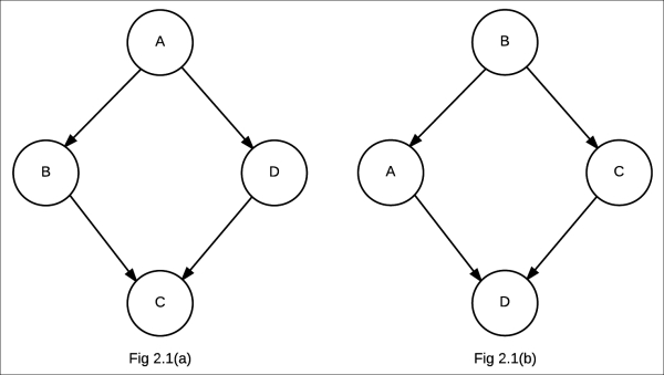
In the preceding figure, the one labeled Fig 2.1(a) is the Bayesian network representing ![]() , whereas the one labeled Fig 2.1(b) is the Bayesian network representing
, whereas the one labeled Fig 2.1(b) is the Bayesian network representing ![]()
The first Bayesian network, Fig 2.1(a), satisfied the first independence assertion, that is, ![]() , but it couldn't satisfy the second one. Similarly, the second Bayesian network, Fig 2.1(b), satisfied the independence assertion
, but it couldn't satisfy the second one. Similarly, the second Bayesian network, Fig 2.1(b), satisfied the independence assertion ![]() , but not the other one. Thus, neither of them is an I-Map for the distribution. Hence, we see that directed models have a limitation and there are conditions that we are unable to represent using directed models.
, but not the other one. Thus, neither of them is an I-Map for the distribution. Hence, we see that directed models have a limitation and there are conditions that we are unable to represent using directed models.
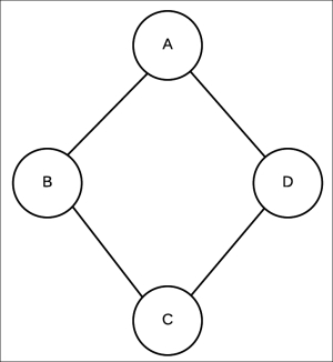
Fig 2.2 Undirected graphical model encoding independencies ![]() and
and ![]()
To correctly represent these independencies, we require an undirected model, also known as a Markov network. These are similar to the Bayesian network, in the sense that we represent all the random variables in the form of nodes, but we represent the dependencies or interaction between these random variables with an undirected edge. Before we go into the representation of these models, we need to think about the parameterization of these models. In the Bayesian network, we had a CPD ![]() associated with every node
associated with every node ![]() . As we don't have any directional influence or a parent-children relationship in the case of the Markov network, instead of using CPDs, we use a more symmetric representation called
factor, which basically represents how likely it is for some states of a variable to agree with the states of other variables.
. As we don't have any directional influence or a parent-children relationship in the case of the Markov network, instead of using CPDs, we use a more symmetric representation called
factor, which basically represents how likely it is for some states of a variable to agree with the states of other variables.
Formally, a factor ![]() of a set of random variables X is defined as a function mapping values of X to some real number
of a set of random variables X is defined as a function mapping values of X to some real number ![]() :
:
Unlike CPDs, there is no notion of directionality or causal relationship among random variables in factors. Factors help in symmetric parameterization of random variables. As the values in a factor don't represent the probability, they are not constrained to sum up to 1 or to be in the range [0,1]. In general, they represent the similarities (or, sometimes, compatibility) among the random variables. Therefore, the higher the value of a combination of states, the greater the compatibility for those states of variables. For example, if we say that two binary random variables A and B are likely to be in the same state rather than different states, we can have a factor where ![]() ,
, ![]() ,
, ![]() , and
, and ![]() . This situation can be represented by a factor as follows:
. This situation can be represented by a factor as follows:
|
A |
B |
|
|---|---|---|
|
|
|
1000 |
|
|
|
1 |
|
|
|
5 |
|
|
|
100 |
We also define the scope of a factor to be the set of random variables over which it is defined. For example, the scope of the preceding factor is {A, B}.
In pgmpy, we can define factors in the following way:
# Firstly we need to import Factor
In [1]: from pgmpy.factors import Factor

# Each factor is represented by its scope,
# cardinality of each variable in the scope and their values
In [2]: phi = Factor(['A', 'B'], [2, 2], [1000, 1, 5, 100])
Now let's try printing a factor:
In [3]: print(phi)
|
a |
b |
phi(A,B) |
|---|---|---|
|
A_0 |
B_0 |
1000.0000 |
|
A_0 |
B_1 |
1.0000 |
|
A_1 |
B_0 |
5.0000 |
|
A_1 |
B_1 |
100.0000 |
Factors subsume the notion of CPD. So, in pgmpy, CPD classes such as TabularCPD, TreeCPD, and RuleCPD are derived from the Factor class.
There are numerous mathematical operations on factors; the major ones are marginalization, reduction, and product.
The marginalization of a factor is similar to its probabilistic marginalization. If we marginalize a factor ![]() whose scope is W with respect to a set of random variables X, it means to sum out all the entries of X, to reduce its scope to
whose scope is W with respect to a set of random variables X, it means to sum out all the entries of X, to reduce its scope to ![]() . Here's an example for marginalizing a factor:
. Here's an example for marginalizing a factor:
# In the preceding example phi, let's try to marginalize it with
# respect to B
In [4]: phi_marginalized = phi.marginalize('B', inplace=False)
In [5]: phi_marginalized.scope()
Out[6]: ['A']
# If inplace=True (default), it would modify the original factor
# instead of returning a new one
In [7]: phi.marginalize('A')
In [8]: print(phi)
╒═════╤═══════════=╕
│ B   │    phi(B)  │
╞═════╪═══════════=╡
│ B_0 │ 1005.0000  │
├─────┼───────────-┤
│ B_1 │  101.0000  │
╘═════╧═══════════=╛

In [9]: phi.scope()
Out[9]: ['B']

# A factor can be also marginalized with respect to more than one # random variable
In [10]: price = Factor(['price', 'quality', 'location'],
                        [2, 2, 2],
                        np.arange(8))
In [11]: price_marginalized = price.marginalize(
                                   ['quality', 'location'],
                                   inplace=False)
In [12]: price_marginalized.scope()
Out[12]: ['price']
In [13]: print(price_marginalized)
╒═════════╤══════════════╕
│ price   │   phi(price) │
╞═════════╪══════════════╡
│ price_0 │       6.0000 │
├─────────┼──────────────┤
│ price_1 │      22.0000 │
╘═════════╧══════════════╛
Reduction of a factor ![]() whose scope is W to the context
whose scope is W to the context ![]() means removing all the entries from the factor where
means removing all the entries from the factor where ![]() . This reduces the scope to
. This reduces the scope to ![]() , as
, as ![]() no longer depends on X.
no longer depends on X.
# In the preceding example phi, let's try to reduce to the context
# of b_0
In [14]: phi = Factor(['a', 'b'], [2, 2], [1000, 1, 5, 100])
In [15]: phi_reduced = phi.reduce(('b', 0), inplace=False)
In [16]: print(phi_reduced)
╒═════╤═══════════╕
│ a   │    phi(a) │
╞═════╪═══════════╡
│ a_0 │ 1000.0000 │
├─────┼───────────┤
│ a_1 │    5.0000 │
╘═════╧═══════════╛

In [17]: phi_reduced.scope()
Out[17]: ['a']

# If inplace=True (default), it would modify the original factor
# instead of returning a new object.
In [18]: phi.reduce(('a', 1))
In [19]: print(phi)
╒═════╤══════════╕
│ b   │   phi(b) │
╞═════╪══════════╡
│ b_0 │   5.0000 │
├─────┼──────────┤
│ b_1 │ 100.0000 │
╘═════╧══════════╛
In [20]: phi.scope()
Out[20]: ['b']

# A factor can be also reduced with respect to more than one
# random variable
In [21]: price_reduced = price.reduce(
                       [('quality', 0), ('location', 1)],
                       inplace=False)
In [22]: price_reduced.scope()
Out[22]: ['price']
The term factor product refers to the product of factors ![]() with a scope X and
with a scope X and ![]() with scope Y to produce a factor
with scope Y to produce a factor ![]() with a scope
with a scope ![]() :
:
In [23]: phi1 = Factor(['a', 'b'], [2, 2], [1000, 1, 5, 100])
In [24]: phi2 = Factor(['b', 'c'], [2, 3],
                       [1, 100, 5, 200, 3, 1000])
# Factors product can be accomplished with the * (product)
# operator
In [25]: phi = phi1 * phi2
In [26]: phi.scope()
Out[26]: ['a', 'b', 'c']
In [27]: print(phi)
╒═════╤═════╤═════╤══════════════╕
│ a   │ b   │ c   │   phi(a,b,c) │
╞═════╪═════╪═════╪══════════════╡
│ a_0 │ b_0 │ c_0 │    1000.0000 │
├─────┼─────┼─────┼──────────────┤
│ a_0 │ b_0 │ c_1 │  100000.0000 │
├─────┼─────┼─────┼──────────────┤
│ a_0 │ b_0 │ c_2 │    5000.0000 │
├─────┼─────┼─────┼──────────────┤
│ a_0 │ b_1 │ c_0 │     200.0000 │
├─────┼─────┼─────┼──────────────┤
│ a_0 │ b_1 │ c_1 │       3.0000 │
├─────┼─────┼─────┼──────────────┤
│ a_0 │ b_1 │ c_2 │    1000.0000 │
├─────┼─────┼─────┼──────────────┤
│ a_1 │ b_0 │ c_0 │       5.0000 │
├─────┼─────┼─────┼──────────────┤
│ a_1 │ b_0 │ c_1 │     500.0000 │
├─────┼─────┼─────┼──────────────┤
│ a_1 │ b_0 │ c_2 │      25.0000 │
├─────┼─────┼─────┼──────────────┤
│ a_1 │ b_1 │ c_0 │   20000.0000 │
├─────┼─────┼─────┼──────────────┤
│ a_1 │ b_1 │ c_1 │     300.0000 │
├─────┼─────┼─────┼──────────────┤
│ a_1 │ b_1 │ c_2 │  100000.0000 │
╘═════╧═════╧═════╧══════════════╛

# or with product method
In [28]: phi_new = phi.product(phi1, phi2)
# would produce a factor with phi_new = phi * phi1 * phi2In the previous section, we saw that we use factors to parameterize a Markov network, which is quite similar to CPDs. Hence, we may think that factors behave in the same way as the CPD. Marginalizing and normalizing it may represent the probability of a variable, but this intuition turns out to be wrong, as we will see in this section. A single factor is just one contribution to the overall joint probability distribution; to have a joint distribution over all the variables, we need the contributions from all the factors of the model. For the dinner example, let's consider the following factors to parameterize the network.
Factor over the variables A and B represented by ![]() :
:
|
A |
B |
|
|---|---|---|
|
|
|
90 |
|
|
|
100 |
|
|
|
1 |
|
|
|
10 |
Factor over the variables B and C represented by ![]() :
:
|
B |
C |
|
|---|---|---|
|
|
|
10 |
|
|
|
80 |
|
|
|
70 |
|
|
|
30 |
Factor over variables C and D represented by ![]() :
:
|
C |
D |
|
|---|---|---|
|
|
|
10 |
|
|
|
1 |
|
|
|
100 |
|
|
|
90 |
Factor over variables A and D represented by ![]() :
:
|
D |
A |
|
|---|---|---|
|
|
|
80 |
|
|
|
60 |
|
|
|
20 |
|
|
|
10 |
Now, considering the preceding factors, let's try to calculate the probability of A by just considering the factor ![]() . On normalizing and marginalizing the factor with respect to B, we get
. On normalizing and marginalizing the factor with respect to B, we get ![]() and
and ![]() . Now, let's try to compute the probability by considering all the factors. To do this, we first need to calculate the factor product of these factors:
. Now, let's try to compute the probability by considering all the factors. To do this, we first need to calculate the factor product of these factors:
|
A |
B |
C |
D |
|
|
|---|---|---|---|---|---|
|
|
|
|
|
|
|
|
|
|
|
|
|
|
|
|
|
|
|
|
|
|
|
|
|
|
|
|
|
|
|
|
|
|
|
|
|
|
|
|
|
|
|
|
|
|
|
|
|
|
|
|
|
|
|
|
|
|
|
|
|
|
|
|
|
|
|
|
|
|
|
|
|
|
|
|
|
|
|
|
|
|
|
|
|
|
|
|
|
|
|
|
|
|
|
|
|
|
|
|
|
|
|
|
|
|
|
|
|
|
|
|
Now, if we normalize and marginalize this factor product, we get ![]() and
and ![]() . Here, we see that there is a huge difference in the probability when we consider only a single factor as compared to when we consider all the factors. Hence, our intuition of factors behaving like CPDs is wrong.
. Here, we see that there is a huge difference in the probability when we consider only a single factor as compared to when we consider all the factors. Hence, our intuition of factors behaving like CPDs is wrong.
Therefore, in a Markov network over a set of variables ![]() having a set of factors
having a set of factors ![]() associated with it, we can compute the joint probability distribution over these variables as follows:
associated with it, we can compute the joint probability distribution over these variables as follows:
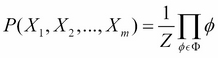
Here, Z is the partition function and ![]() .
.
Also, a distribution ![]() is called a Gibbs distribution parameterized by a set of factors
is called a Gibbs distribution parameterized by a set of factors ![]() if it is defined as follows:
if it is defined as follows:
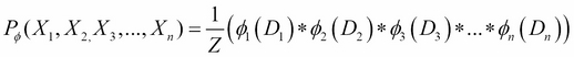
Here, ![]() is a normalizing constant called the partition function.
is a normalizing constant called the partition function.
To construct a Markov network, we need to associate the parameterization of a Gibbs distribution to the set of factors of an undirected graph structure. A factor with the X and Y scopes represents a direct relationship between them.
Let's see how we can represent a Markov model using pgmpy:
# First import MarkovModel class from pgmpy.models
In [1]: from pgmpy.models import MarkovModel
In [2]: model = MarkovModel([('A', 'B'), ('B', 'C')])
In [3]: model.add_node('D')
In [4]: model.add_edges_from([('C', 'D'), ('D', 'A')])
Now, let's try to define a few factors to associate with this model:
In [5]: from pgmpy.factors import Factor
In [6]: factor_a_b = Factor(variables=['A', 'B'],
                            cardinality=[2, 2],
                            value=[90, 100, 1, 10])
In [7]: factor_b_c = Factor(variables=['B', 'C'],
                            cardinality=[2, 2],
                            value=[10, 80, 70, 30])
In [8]: factor_c_d = Factor(variables=['C', 'D'],
                            cardinality=[2, 2],
                            value=[10, 1, 100, 90])
In [9]: factor_d_a = Factor(variables=['D', 'A'],
                            cardinality=[2, 2],
                            value=[80, 60, 20, 10])
We can associate the factors to the model using the add_factors method:
In [10]: model.add_factors(factor_a_b, factor_b_c,
                           factor_c_d, factor_d_a)
In [11]: model.get_factors()
Out[11]:
[<Factor representing phi(A:2, B:2) at 0x7f18504477b8>,
 <Factor representing phi(B:2, C:2) at 0x7f18504479b0>,
 <Factor representing phi(C:2, D:2) at 0x7f1850447f98>,
 <Factor representing phi(D:2, A:2) at 0x7f1850455358>]