
In the earlier section, we discussed a variant of belief propagation where we relaxed the constraint of having a clique tree, and did belief propagation on a cluster graph. In this section, we will take a different approach. Instead of relaxing on the structure, we will be approximating the messages passed between the clusters. Although this approach can be extended to work with cluster graphs as well, the scope of this book is only limited to clique trees.
Let's consider a simple pairwise Markov model, as shown in Fig 4.9. As discussed in the previous section, a pairwise Markov model is simply a Markov model with the factors ![]() associated with each edge
associated with each edge ![]() , along with the univariate factors
, along with the univariate factors ![]() corresponding to each random variable
corresponding to each random variable ![]() . Thus, the following model will have factors such as
. Thus, the following model will have factors such as ![]() ,
, ![]() , and
, and ![]() along with
along with ![]() ,
, ![]() ,
, ![]() , and so on. Let's also assume that each random variable present in this network is binary.
, and so on. Let's also assume that each random variable present in this network is binary.
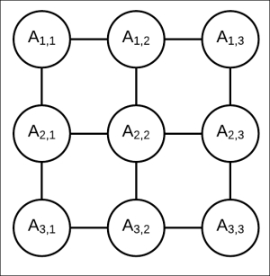
Fig 4.9: Markov model represented by 3 x 3 grid network
A cluster tree for this network can be created, as shown in Fig 4.10. Although this may not be an optimal cluster tree, it's a valid one as it satisfies the running intersection property, and each node represents a cluster of random variables present in the original network.
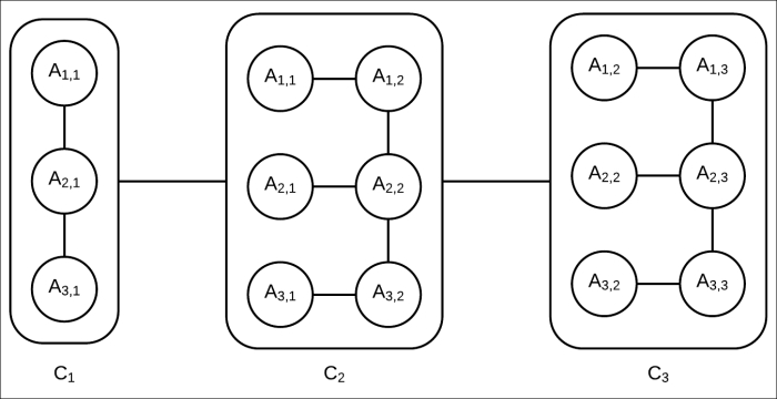
Fig 4.10: Cluster tree corresponding to the Markov model in Fig 4.9
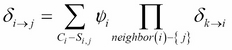
In our previous discussion about the cluster tree (or clique tree), we never discussed the internal structure of each cluster, but the internal structure of the cluster becomes important in the context of this algorithm. For the calibration of the previously mentioned clique tree, we need to transmit message across the clusters. Suppose the message from ![]() to
to ![]() , that is
, that is ![]() , can be approximated by its factored form as follows:
, can be approximated by its factored form as follows:
We can see that the factored form is more compact as compared to the original message. The original message will have ![]() variables, whereas the factored form can be represented only by using 2 * 3 = 6 parameters (two parameters for each variable as they are assumed to be binary). However, this compact representation helps us to save only two variables. So, the question that arises is whether the approximation is worth the savings or not. How can we use these approximations to compute the inference? We can get similar saving even if we just use some approximation that is richer than the naive independence assumption we used earlier. Even if we use approximations by exploiting the conditional independence among the random variables represented by the chain structure
variables, whereas the factored form can be represented only by using 2 * 3 = 6 parameters (two parameters for each variable as they are assumed to be binary). However, this compact representation helps us to save only two variables. So, the question that arises is whether the approximation is worth the savings or not. How can we use these approximations to compute the inference? We can get similar saving even if we just use some approximation that is richer than the naive independence assumption we used earlier. Even if we use approximations by exploiting the conditional independence among the random variables represented by the chain structure ![]() , the question still remains the same: how can we use these approximations to compute the inference?
, the question still remains the same: how can we use these approximations to compute the inference?
Before answering these questions, let's discuss factor sets. A factor set ![]() provides a compact representation of
provides a compact representation of ![]() . Thus, the product of two factor sets is nothing but their union. For example, suppose
. Thus, the product of two factor sets is nothing but their union. For example, suppose ![]() and
and ![]() . Then, their product should be
. Then, their product should be ![]() , which can be written as a factor set of
, which can be written as a factor set of ![]() .
.
Coming back to our previous question, how can we use these approximations to compute the inference? Let's assume that we somehow factorized the message from cluster ![]() to cluster
to cluster ![]() , that is
, that is ![]() into a factor set
into a factor set ![]() consisting of univariate factors. Similarly, consider that we factorized the message from cluster
consisting of univariate factors. Similarly, consider that we factorized the message from cluster ![]() to cluster
to cluster ![]() , and
, and ![]() into a factor set
into a factor set ![]() consisting only of univariate terms. To compute the belief of cluster
consisting only of univariate terms. To compute the belief of cluster ![]() , we need to multiply the initial potential of
, we need to multiply the initial potential of ![]() , that is
, that is ![]() with messages
with messages ![]() and
and ![]() . As both the messages
. As both the messages ![]() and
and ![]() have been factored into factor sets consisting only of univariate factors, the network structure of cluster
have been factored into factor sets consisting only of univariate factors, the network structure of cluster ![]() remains unchanged (as shown in Fig 4.11). That is, no extra edge between any two variables is added as none of the factors from the message represent interaction among the random variables:
remains unchanged (as shown in Fig 4.11). That is, no extra edge between any two variables is added as none of the factors from the message represent interaction among the random variables:
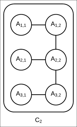
Fig 4.11: Internal network structure of cluster ![]() remains unchanged. It is still a tree with tree width of two.
remains unchanged. It is still a tree with tree width of two.
As the cluster ![]() has a tree structure internally, we can apply any exact inference algorithm to compute the marginals of the random variables present in this cluster.
has a tree structure internally, we can apply any exact inference algorithm to compute the marginals of the random variables present in this cluster.
If we use a richer approximation that exploits the chain structure of the cluster ![]() to compute the message
to compute the message ![]() , it will contain factors representing interactions among
, it will contain factors representing interactions among ![]() ,
, ![]() and
and ![]() ,
, ![]() . When this message is multiplied with
. When this message is multiplied with ![]() along with
along with ![]() , it will modify the network structure of
, it will modify the network structure of ![]() ; it will introduce an edge between
; it will introduce an edge between ![]() as well as an edge between
as well as an edge between ![]() , as shown in Fig 4.12. Still, the network has a tree width of two and we can still use exact inference to compute the marginals of the random variables present in this cluster.
, as shown in Fig 4.12. Still, the network has a tree width of two and we can still use exact inference to compute the marginals of the random variables present in this cluster.
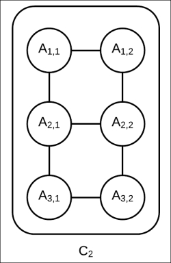
Fig 4.12: The internal network structure of ![]() with a richer approximation of
with a richer approximation of ![]()
So we can see how these approximations can help us in computing the inference.
Now, the question is, how do we compute these messages, or more precisely, how do we factorize the message from cluster ![]() to
to ![]() , that is
, that is ![]() , into factor sets?
, into factor sets?
To answer this question, let's go back to the first principle method of computing a message from ![]() to
to ![]() .
. ![]() is computed as follows:
is computed as follows:
If all the messages from neighbors ![]() are already factorized into factor sets, then their product is nothing but the union of their corresponding factor sets. The initial potential
are already factorized into factor sets, then their product is nothing but the union of their corresponding factor sets. The initial potential ![]() can be factorized into a factor set of all the initial factors present in the cluster. The final factor product can be computed by the union of all the factor sets.
can be factorized into a factor set of all the initial factors present in the cluster. The final factor product can be computed by the union of all the factor sets.
To compute the message, we also need to marginalize the after-product. To marginalize a factor set ![]() with respect to a variable X, we need to couple all the factors containing X and marginalize them. So, like the product of a factor set, marginalizing it doesn't present any problems. So, the major problem lies in factorizing the marginal probabilities into a factor set. In a clique tree, the results from marginalizing a clique would not satisfy any conditional independence, so it can't be factorized into a factor set. However, for efficient inference, we want the messages to be factorized into a factor set. This can be achieved by approximating the message by a family of distributions that can be factorized. It turns out that there is a family of distributions that can be approximated for these messages and that the distribution is simply the product of the marginals of the individual variables present in the messages. The message is often not normalized, so it is not treated as a distribution. However, we can normalize the message and treat it as a distribution. To compute the marginals, we can use any of the exact inference algorithms that we discussed earlier, such as variable elimination or belief propagation.
with respect to a variable X, we need to couple all the factors containing X and marginalize them. So, like the product of a factor set, marginalizing it doesn't present any problems. So, the major problem lies in factorizing the marginal probabilities into a factor set. In a clique tree, the results from marginalizing a clique would not satisfy any conditional independence, so it can't be factorized into a factor set. However, for efficient inference, we want the messages to be factorized into a factor set. This can be achieved by approximating the message by a family of distributions that can be factorized. It turns out that there is a family of distributions that can be approximated for these messages and that the distribution is simply the product of the marginals of the individual variables present in the messages. The message is often not normalized, so it is not treated as a distribution. However, we can normalize the message and treat it as a distribution. To compute the marginals, we can use any of the exact inference algorithms that we discussed earlier, such as variable elimination or belief propagation.
Summarizing all these points, we can create an algorithm to compute the approximate messages to be transmitted between clusters in the clique tree:
- Create a factor set
 by the union of all the factor sets corresponding to the initial cluster potential as well as the input messages received.
-
Initialize an inference data structure
 with this factor set to perform exact inference. It could be a clique tree in the case of belief propagation or a set of factors in the case of variable elimination.
-
Perform inference on to compute the marginals of variables to be present in the final message.
- The factor set of the marginals is the output message.
For example, let's try to work out how to create the messages ![]() and
and ![]() for the cluster tree represented in Fig 4.11, starting with
for the cluster tree represented in Fig 4.11, starting with ![]() . This can be computed by creating a factor set
. This can be computed by creating a factor set ![]() as the union of
as the union of ![]() (factor set corresponding to
(factor set corresponding to ![]() ) and the input message. As there is no input message for this cluster,
) and the input message. As there is no input message for this cluster, ![]() will be
will be ![]() . To compute the marginals for
. To compute the marginals for ![]() ,
, ![]() , and
, and ![]() using the belief propagation method, we could use a clique tree, as shown in Fig 4.13:
using the belief propagation method, we could use a clique tree, as shown in Fig 4.13:
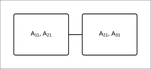
Fig 4.13: A Clique tree to compute the marginals of ![]() ,
, ![]() , and
, and ![]()
The factor set representing the message from ![]() to
to ![]() , that is
, that is ![]() , formed by the marginals of
, formed by the marginals of ![]() ,
, ![]() , and
, and ![]() will be
will be ![]() .
.
Similarly, to compute ![]() , the first step is to create
, the first step is to create ![]() , where
, where ![]() represents the factor set corresponding to
represents the factor set corresponding to ![]() . Then, we create an inference data structure for exact inference to compute the marginals of
. Then, we create an inference data structure for exact inference to compute the marginals of ![]() ,
, ![]() , and
, and ![]() and initialize with
and initialize with ![]() . As
. As ![]() contains only univariate factors, the structure of
contains only univariate factors, the structure of ![]() remains unchanged. Fig 4.14 represents the clique tree that can be used as an inference data structure to compute the marginals of
remains unchanged. Fig 4.14 represents the clique tree that can be used as an inference data structure to compute the marginals of ![]() ,
, ![]() , and
, and ![]() :
:
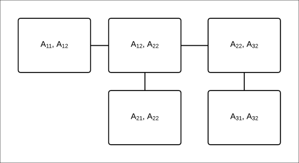
Fig 4.14: A clique tree to compute the marginals of ![]() ,
, ![]() , and
, and ![]()
In the previous section, we discussed the methods of creating messages to transmit between clusters. Once we have these messages, the next task is to perform inference on the clique tree. While discussing exact inference, we discussed two methods of performing inference on a clique tree, one being the sum-product algorithm, the other being the sum-product-divide or belief update algorithm. For the exact inference, both of these algorithms will give the same result, but in the case of approximate inference, they are not the same.
Before we discuss these steps in detail, let's look at the difference between the exact and approximate inference algorithms. Once the tree is calibrated, the beliefs so computed don't represent the joint probability distribution of all the variables present in the cluster (as it was in the case of exact inference). So, to answer queries about the variables present in the cluster, we can't just marginalize other variables from the belief. Instead, after calibration, we have the factor sets of beliefs parameterizing the network structure of the corresponding cluster. In the previous example, after the clique tree is calibrated, the belief for the cluster ![]() can be factorized as follows:
can be factorized as follows:
The factors present in the factor set ![]() parameterize the network structure of cluster
parameterize the network structure of cluster ![]() . As the network structure allows tractable inference, we can answer queries about these variables using inference methods such as variable elimination or belief propagation.
. As the network structure allows tractable inference, we can answer queries about these variables using inference methods such as variable elimination or belief propagation.
The sum-product expectation propagation algorithm is similar to the sum-product algorithm we discussed for exact inference, except that we modify the procedure to compute the message. There, we computed the message by summing out (or marginalizing) the variable from the product of factors. Here, we compute the message as discussed in the previous section. Similar to the exact inference equivalent, in the case of approximate inference for calibration of the clique tree, we require two passes, one upward and one downward. So, unlike the previous approximate inference, it converges in a fixed number of steps.
Let's start with a simple example, as shown in Fig 4.15:
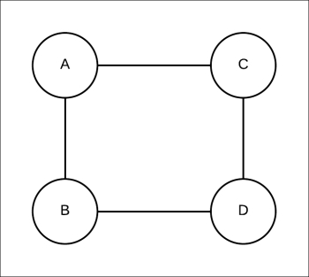
Fig 4.15: Simple pairwise Markov network consisting of four random variables
Suppose the factors associated with the given Markov model are as follows:
|
A |
B |
|
|---|---|---|
|
|
|
10 |
|
|
|
0.1 |
|
|
|
0.1 |
|
|
|
10 |
|
A |
C |
|
|---|---|---|
|
|
|
5 |
|
|
|
0.2 |
|
|
|
0.2 |
|
|
|
5 |
|
C |
D |
|
|---|---|---|
|
|
|
0.5 |
|
|
|
1 |
|
|
|
20 |
|
|
|
2.5 |
|
D |
B |
|
|---|---|---|
|
|
|
5 |
|
|
|
0.2 |
|
|
|
0.2 |
|
|
|
5 |
From the preceding factors, we can see that there is a strong coupling between the variables A and B. It seems that A = B. The potentials ![]() and
and ![]() indicate weaker coupling between A and C, and B and D.
indicate weaker coupling between A and C, and B and D.
If we perform the exact inference in this network, we find the following marginal posteriors:
Let's try to compute the marginals using the approximate inference method that we discussed now using pgmpy. The clique tree constructed is shown in Fig 4.16:
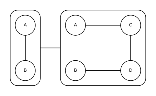
Fig 4.16: The clique tree constructed for the Markov model represented in Fig 4.18
In [1]: from pgmpy.factors import Factor
In [2]: from pgmpy.factors import FactorSet
In [3]: from pgmpy.models import MarkovModel
In [4]: from pgmpy.inference import VariableElimination
In [5]: from pgmpy.inference import BeliefPropagation
In [6]: import functools
In [7]: def compute_message(cluster_1, cluster_2,
                            inference_data_structure=
                                VariableElimination):
    """
       Computes the message from cluster_1 to cluster_2.
    The messages are computed by projecting a factor set to
    produce a set of marginals over a given set of scopes. The
    factor set is nothing but the factors present in the models.

       The algorithm for computing messages between any two clusters
    is:
    * Build an inference data structure with all the factors
      represented in the cluster.
    * Perform inference on the cluster using the inference data
      structure to compute the marginals of the variables present
      in the sepset between these two clusters.
       * The output message is the factor set of all the computed
         marginals.

       Parameters
    ----------
    cluster_1: MarkovModel, BayesianModel, or any pgmpy supported
               graphical model
                  The cluster producing the message
    cluster_2: MarkovModel, BayesianModel, or any pgmpy supported
               graphical model
               The cluster receiving the message

       inference_data_structure: Inference class such as
                             VariableElimination or BeliefPropagation
                  The inference data structure used to produce factor
                  set of marginals
    """
    # Sepset variables between the two clusters
    sepset_var = set(cluster_1.nodes()).intersection(
                                            cluster_2.nodes())

    # Initialize the inference data structure
    inference = inference_data_structure(cluster_1)

    # Perform inference
    query = inference.query(list(sepset_var))

    # The factor set of all the computed messages is the output
    # message query would be a dictionary with key as the variable
    # and value as the corresponding marginal thus the values
    # would represent the factor set
       return FactorSet(*query.values())

In [8]: def compute_belief(cluster, *input_factored_messages):
       """
       Computes the belief a particular cluster given the cluster
       and input messages

       delta_{j
ightarrow i} where j are all the neighbors of
       cluster i. The cluster belief is computed as:
    .. math::
      eta_i = psi_i prod_{j in Nb_i} delta_{j
ightarrow i}

    where psi_i is the cluster potential. As the cluster belief
    represents the probability and it should be normalized to sum
    up to 1.

    Parameters
    ----------
    cluster: MarkovModel, BayesianModel, or any pgmpy supported
             graphical model
            The cluster whose cluster potential is going to be
            computed.
   *input_factored_messages: FactorSet or a group of FactorSets
            All the input messages to the clusters. They should be
            factor sets

    Returns
    -------
    cluster_belief: Factor
        The cluster belief of the corresponding cluster
    """
    messages_prod = functools.reduce(lambda x, y: x * y,
                            input_factored_messages)

    # As messages_prod would be a factor set, so its corresponding
    # factor would be product of all the factors present in the
    # factorset
    messages_prod_factor = functools.reduce(lambda x, y: x * y,
                            messages_prod.factors)

    # Computing cluster potential psi
    psi = functools.reduce(lambda x, y: x * y,
                           cluster.get_factors())

    # As psi represents the probability it should be normalized
    psi.normalize()

    # Computing the cluster belief according the formula stated
    # above
    cluster_belief = psi * messages_prod_factor

    # As cluster belief represents a probability distribution in
    # this case, thus it should be normalized
    cluster_belief.normalize()

    return cluster_belief

In [9]: phi_a_b = Factor(['a', 'b'], [2, 2], [10, 0.1, 0.1, 10])
In [10]: phi_a_c = Factor(['a', 'c'], [2, 2], [5, 0.2, 0.2, 5])
In [11]: phi_c_d = Factor(['c', 'd'], [2, 2], [0.5, 1, 20, 2.5])
In [12]: phi_d_b = Factor(['d', 'b'], [2, 2], [5, 0.2, 0.2, 5])

# Cluster 1 is a MarkovModel A--B
In [13]: cluster_1 = MarkovModel([('a', 'b')])

# Adding factors
In [14]: cluster_1.add_factors(phi_a_b)

# Cluster 2 is a MarkovModel A--C--D--B
In [15]: cluster_2 = MarkovModel([('a', 'c'), ('c', 'd'),
                                  ('d', 'b')])

# Adding factors
In [16]: cluster_2.add_factors(phi_a_c, phi_c_d, phi_d_b)

# Message passed from cluster 1 -> 2 should the M-Projection of psi1
# as the sepset of cluster 1 and 2 is A, B thus there is no need to
# marginalize psi1
In [17]: delta_1_2 = compute_message(cluster_1, cluster_2)

# If we want to use any other inference data structure we can pass
# them as an input argument such as: delta_1_2 =
# compute_message(cluster_1, cluster_2, BeliefPropagation)
In [18]: beta_2 = compute_belief(cluster_2, delta_1_2)
In [19]: print(beta_2.marginalize(['a', 'b'], inplace=False))

     ╒═════╤═════╤════════════╕

     │ c   │ d   │   phi(c,d) │

     ╞═════╪═════╪════════════╡

     │ c_0 │ d_0 │     0.0208 │

     ├─────┼─────┼────────────┤

     │ c_0 │ d_1 │     0.0417 │

     ├─────┼─────┼────────────┤

     │ c_1 │ d_0 │     0.8333 │

     ├─────┼─────┼────────────┤

     │ c_1 │ d_1 │     0.1042 │

     ╘═════╧═════╧════════════╛

# Lets compute the belief of cluster1, first we need to compute the
# output message from cluster 2 to cluster 1
In [20]: delta_2_1 = compute_message(cluster_2, cluster_1)

# Lets see the distribution of both of these variables in the
# computed message
In [21]: for phi in delta_2_1.factors:
             print(phi)

     ╒═════╤══════════╕

     │ b   │   phi(b) │

     ╞═════╪══════════╡

     │ b_0 │   0.8269 │

     ├─────┼──────────┤

     │ b_1 │   0.1731 │

     ╘═════╧══════════╛

     ╒═════╤══════════╕

     │ a   │   phi(a) │

     ╞═════╪══════════╡

     │ a_0 │   0.0962 │

     ├─────┼──────────┤

     │ a_1 │   0.9038 │

     ╘═════╧══════════╛

# The belief of cluster1 would be
In [22]: beta_1 = compute_belief(cluster_1, delta_2_1)
In [23]: print(beta_1)

     ╒═════╤═════╤════════════╕

     │ a   │ b   │   phi(a,b) │

     ╞═════╪═════╪════════════╡

     │ a_0 │ b_0 │     0.3264 │

     ├─────┼─────┼────────────┤

     │ a_0 │ b_1 │     0.0007 │

     ├─────┼─────┼────────────┤

     │ a_1 │ b_0 │     0.0307 │

     ├─────┼─────┼────────────┤

     │ a_1 │ b_1 │     0.6422 │

     ╘═════╧═════╧════════════╛
Let's start with ![]() . It can be computed by marginalizing
. It can be computed by marginalizing ![]() with respect to A and B. Normalizing the messages to treat it as a distribution, we get
with respect to A and B. Normalizing the messages to treat it as a distribution, we get ![]() and
and ![]() . Similarly, for B we get
. Similarly, for B we get ![]() ,
, ![]() . Thus,
. Thus, ![]() or to put
or to put ![]() would be as follows:
would be as follows:
However, from exact inference we know the following:
We see that the approximate message loses the coupling between A and B. Thus, it is a poor approximation of the exact message. The problem with this approach is that the approximation of the message is done considering the impact of this message on the downstream cluster.
Similarly, if we compute ![]() , we get
, we get ![]() and
and ![]() . This is again in contrast with the factor
. This is again in contrast with the factor ![]() , which strongly suggests that A= B. When we combine the message with
, which strongly suggests that A= B. When we combine the message with ![]() , we get the belief for the cluster
, we get the belief for the cluster ![]() as follows:
as follows:
As we have seen in the previous example, when we had the message ![]() , we computed the posterior probability of A and B fairly close to the exact value. This raises the question, can we use the newly computed posterior probability to correctly approximate the message
, we computed the posterior probability of A and B fairly close to the exact value. This raises the question, can we use the newly computed posterior probability to correctly approximate the message ![]() ? The answer is, no, we can't. The reason for this is that, if we use the information that we got from
? The answer is, no, we can't. The reason for this is that, if we use the information that we got from ![]() and use it to correct
and use it to correct ![]() , we will be double-counting evidence. So, is there a way to get away with this double-counting yet still use the information?
, we will be double-counting evidence. So, is there a way to get away with this double-counting yet still use the information?
If you recall, in the previous chapter, we discussed the belief update method that we used to compute the message from the cluster ![]() to the cluster
to the cluster ![]() as follows:
as follows:
So, using the belief update propagation, we can use the information ![]() to modify
to modify ![]() . Let's see how to use it in the case of factor sets. The preceding equation can be translated for the factor set as follows:
. Let's see how to use it in the case of factor sets. The preceding equation can be translated for the factor set as follows:
Here, ![]() approximates the belief of the cluster
approximates the belief of the cluster ![]() by a family of distributions that can be factorized. This is similar to what we did in the case of approximating a message by a family of factorized distributions. Let's go back to the example again to see how to implement it.
by a family of distributions that can be factorized. This is similar to what we did in the case of approximating a message by a family of factorized distributions. Let's go back to the example again to see how to implement it.
First, initialize all the messages to 1. In the first iteration, the value of ![]() is the same as what we computed earlier as
is the same as what we computed earlier as ![]() is 1 and so would be
is 1 and so would be ![]() . In the second iteration to compute
. In the second iteration to compute ![]() , we will be using the value of
, we will be using the value of ![]() . Marginalizing
. Marginalizing ![]() with respect to B, we get
with respect to B, we get ![]() equals 0.326 + 0.001 = 0.327 and
equals 0.326 + 0.001 = 0.327 and ![]() equals 0.031+ 0.642 = 0.673. Similarly, marginalizing
equals 0.031+ 0.642 = 0.673. Similarly, marginalizing ![]() with respect to B, we get
with respect to B, we get ![]() and
and ![]() . So,
. So, ![]() will be as follows:
will be as follows:
can be computed by dividing ![]() with
with ![]() . Finally, we have to normalize
. Finally, we have to normalize ![]() to treat it as a distribution.
to treat it as a distribution.
The newly formed ![]() can be viewed as a correction for
can be viewed as a correction for ![]() in the next iteration, and so, it will be
in the next iteration, and so, it will be ![]() for
for ![]() . So, unlike the previous method, it doesn't converge in two steps; rather it requires multiple iterations of message passing between the two clusters, each correcting the other.
. So, unlike the previous method, it doesn't converge in two steps; rather it requires multiple iterations of message passing between the two clusters, each correcting the other.
In the previous chapter, we studied MAP inference using variable elimination and max-product message passing in clique trees. In a similar fashion, we can apply max-product message passing on the cluster graph.
Recall that in the case of clique trees, the max-product message passing was analogous to their sum-product message passing algorithm, differing only in the way the message was computed. We used the maximization operation instead of summation. Also, in the case of cluster trees, the max-product message passing is analogous to their sum-product counterpart, maximizing the variable instead of summing it out. Unlike their sum-product counterpart, there is no guarantee of the convergence of this algorithm; it is more susceptible to nonconvergence. One reason for this is that the summation averages the messages, whereas maximization doesn't. Thus, it can't reduce oscillations.
Before going into further discussion about max-product message passing in cluster trees, let's discuss local optimality and decoding. We say that an assignment ![]() has the local optimality property, if for each clique
has the local optimality property, if for each clique ![]() in a max-calibrated clique tree, we have the following:
in a max-calibrated clique tree, we have the following:
The assignment to ![]() in
in ![]() optimizes the belief of
optimizes the belief of ![]() (that is
(that is ![]() ). The task of finding a locally optimal assignment
). The task of finding a locally optimal assignment ![]() , given a max-calibrated set of beliefs is known as decoding.
, given a max-calibrated set of beliefs is known as decoding.
Just like the sum-product message passing on cluster trees, the max-product message passing will not give the exact max-marginal even after max-calibration. The beliefs so formed after max-calibration are called pseudo max-marginals.
Once we have the pseudo max-marginals by max-product message passing, we are left with the task of decoding these marginals. As discussed earlier, the task of decoding is nothing but finding a locally optimal assignment, and unlike clique trees, such assignments do not necessarily exist in the case of cluster graphs. Let's look at a simple example. Consider the cluster graph shown in Fig 4.17:
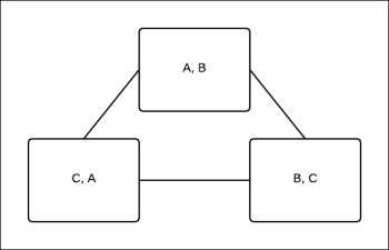
Fig 4.17: The cluster graph of three random variables A, B, and C
The beliefs after max-calibration are as follows:
|
A |
B |
|
|---|---|---|
|
|
|
1 |
|
|
|
2 |
|
|
|
2 |
|
|
|
1 |
|
B |
C |
|
|---|---|---|
|
|
|
1 |
|
|
|
2 |
|
|
|
2 |
|
|
|
1 |
|
A |
C |
|
|---|---|---|
|
|
|
1 |
|
|
|
2 |
|
|
|
2 |
|
|
|
1 |
For example, to maximize ![]() , we can select the value of
, we can select the value of ![]() ,
, ![]() . Thus, to maximize the belief
. Thus, to maximize the belief ![]() , we have to select
, we have to select ![]() . Now, we can see that the assignments
. Now, we can see that the assignments ![]() and
and ![]() do not correspond to the maximum value of belief
do not correspond to the maximum value of belief ![]() . No matter which assignment we choose, we can't obtain a single joint assignment that maximizes all three beliefs. These kinds of loops are called frustrating loops.
. No matter which assignment we choose, we can't obtain a single joint assignment that maximizes all three beliefs. These kinds of loops are called frustrating loops.
From the preceding example, we can create a simple hypothesis that if all the node beliefs are ambiguous, then there is no locally optimal joint assignment, but this is not always true. Let's take the example of the following beliefs:
|
A |
B |
|
|---|---|---|
|
|
|
2 |
|
|
|
1 |
|
|
|
1 |
|
|
|
2 |
|
B |
C |
|
|---|---|---|
|
|
|
2 |
|
|
|
1 |
|
|
|
1 |
|
|
|
2 |
|
A |
C |
|
|---|---|---|
|
|
|
2 |
|
|
|
1 |
|
|
|
1 |
|
|
|
2 |
We can see that assignments ![]() ,
, ![]() , and
, and ![]() , as well as
, as well as ![]() ,
, ![]() , and
, and ![]() are locally optimal.
are locally optimal.
We saw some cases where there are no locally optimal assignments and there are cases where we can find locally optimal assignments. So, the basic question that arises is, how do we find locally optimal assignments, if any exist?
From the definition of local optimality, we can say that an assignment is locally optimal if and only if it selects optimal assignments from each cluster. Keeping this in mind, we can now assign labels to each assignment in a cluster. The label of the assignment can be "legal", if it optimizes the belief of that cluster, or "illegal" if it doesn't. So now, the decoding task is converted into a task of finding an assignment such that it is the legal value for all the clusters. This is nothing but a constraint satisfaction problem, where the constraints are obtained from the local optimality. The detailed survey of the constrained satisfaction problem is beyond the scope of this book. Thus, given a max-product calibrated cluster graph, we can convert it into a constrained satisfaction problem (CSP) simply by taking the belief of each cluster, and changing each assignment that locally optimizes the belief to 1 and the rest to 0. We then run a CSP solution method. If the outcome is an assignment that achieves 1 in every cluster belief, then the assignment is guaranteed to be a locally optimal assignment. For example, one of the CSP solution methods can be defined in terms of the Markov network, where all the entries are either 1 for legal assignments or 0 for illegal ones. Thus, CSP is simply finding the MAP assignment in a Markov model with {0, 1} valued beliefs. The CSP problem is itself an NP-hard problem. Thus, we can't guarantee that we would be able to find a locally optimal assignment efficiently, even if it existed.
The following is the implementation using pgmpy:
In [1]: from pgmpy.models import BayesianModel
In [2]: from pgmpy.factors import TabularCPD
In [3]: from pgmpy.inference import ClusterBeliefPropagation as
        CBP

# Create a bayesian model as we did in the previous chapters
In [4]: model = BayesianModel([
                     ('rain', 'traffic_jam'),
                     ('accident', 'traffic_jam'),
                     ('traffic_jam', 'long_queues'),
                     ('traffic_jam', 'late_for_school'),
                     ('getting_up_late', 'late_for_school')])
In [5]: cpd_rain = TabularCPD('rain', 2, [[0.4], [0.6]])
In [6]: cpd_accident = TabularCPD('accident', 2, [[0.2], [0.8]])
In [7]: cpd_traffic_jam = TabularCPD(
                            'traffic_jam', 2,
                            [[0.9, 0.6, 0.7, 0.1],
                             [0.1, 0.4, 0.3, 0.9]],
                            evidence=['rain', 'accident'],
                            evidence_card=[2, 2])
In [8]: cpd_getting_up_late = TabularCPD('getting_up_late', 2,
                                         [[0.6], [0.4]])
In [9]: cpd_late_for_school = TabularCPD(
                            'late_for_school', 2,
                            [[0.9, 0.45, 0.8, 0.1],
                             [0.1, 0.55, 0.2, 0.9]],
                            evidence = ['getting_up_late',
                                        'traffic_jam'],
                            evidence_card=[2, 2])
In [10]: cpd_long_queues = TabularCPD('long_queues', 2,
                                      [[0.9, 0.2],
                                       [0.1, 0.8]],
                                      evidence=['traffic_jam'],
                                      evidence_card=[2])
In [11]: model.add_cpds(cpd_rain, cpd_accident, cpd_traffic_jam,
                        cpd_getting_up_late, cpd_late_for_school,
                        cpd_long_queues)
In [12]: cbp_inference = CBP(model)
In [13]: cbp_inference.map_query(variables=['traffic_jam',
                                            'late_for_school'])
In [14]: cbp_inference.map_query(variables=['traffic_jam'],
                                 evidence={'accident': 1,
                                           'long_queues': 0})