
Chapter 6: Music and Text Generation with PyTorch
PyTorch is a fantastic tool for both researching deep learning models and developing deep learning-based applications. In the previous chapters, we looked at model architectures across various domains and model types. We used PyTorch to build these architectures from scratch and used pre-trained models from the PyTorch model zoo. We will switch gears from this chapter onward and dive deep into generative models.
In the previous chapters, most of our examples and exercises revolved around developing models for classification, which is a supervised learning task. However, deep learning models have also proven extremely effective when it comes to unsupervised learning tasks. Deep generative models are one such example. These models are trained using lots of unlabeled data. Once trained, the model can generate similar meaningful data. It does so by learning the underlying structure and patterns in the input data.
In this chapter, we will develop text and music generators. For developing the text generator, we will utilize the transformer-based language model we trained in Chapter 5, Hybrid Advanced Models. We will extend the transformer model using PyTorch so that it works as a text generator. Furthermore, we will demonstrate how to use advanced pre-trained transformer models in PyTorch in order to set up a text generator in a few lines of code. Finally, we will build a music generator model that's been trained on an MIDI dataset from scratch using PyTorch.
By the end of this chapter, you should be able to create your own text and music generation models in PyTorch. You will also be able to apply different sampling or generation strategies to generate data from such models. This chapter covers the following topics:
- Building a transformer-based text generator with PyTorch
- Using a pre-trained GPT 2 model as a text generator
- Generating MIDI music with LSTMs using PyTorch
Technical requirements
We will be using Jupyter notebooks for all our exercises. The following is a list of Python libraries that you need to install for this chapter using pip; for example, run pip install torch==1.4.0 on the command line:
jupyter==1.0.0
torch==1.4.0
tqdm==4.43.0
matplotlib==3.1.2
torchtext==0.5.0
transformers==3.0.2
scikit-image==0.14.2
All the code files that are relevant to this chapter are available at https://github.com/PacktPublishing/Mastering-PyTorch/tree/master/Chapter06.
Building a transformer-based text generator with PyTorch
We built a transformer-based language model using PyTorch in the previous chapter. Because a language model models the probability of a certain word following a given sequence of words, we are more than half-way through in building our own text generator. In this section, we will learn how to extend this language model as a deep generative model that can generate arbitrary yet meaningful sentences, given an initial textual cue in the form of a sequence of words.
Training the transformer-based language model
In the previous chapter, we trained a language model for 5 epochs. In this section, we will follow those exact same steps but will train the model for longer; that is, 50 epochs. The goal here is to obtain a better performing language model that can then generate realistic sentences. Please note that model training can take several hours. Hence, it is recommended to train it in the background; for example, overnight. In order to follow the steps for training the language model, please follow the complete code at https://github.com/PacktPublishing/Mastering-PyTorch/blob/master/Chapter06/text_generation.ipynb.
Upon training for 50 epochs, we get the following output:

Figure 6.1 – Language model training logs
Now that we have successfully trained the transformer model for 50 epochs, we can move on to the actual exercise, where we will extend this trained language model as a text generation model.
Saving and loading the language model
Here, we will simply save the best performing model checkpoint once the training is complete. We can then separately load this pre-trained model:
- Once the model has been trained, it is ideal to save it locally so that you avoid having to retrain it from scratch. You can save it as follows:
mdl_pth = './transformer.pth'
torch.save(best_model_so_far.state_dict(), mdl_pth)
- We can now load the saved model so that we can extend this language model as a text generation model:
# load the best trained model
transformer_cached = Transformer(num_tokens, embedding_size, num_heads, num_hidden_params, num_layers, dropout).to(device)
transformer_cached.load_state_dict(torch.load(mdl_pth))
In this section, we re-instantiated a transformer model object and then loaded the pre-trained model weights into this new model object. Next, we will use this model to generate text.
Using the language model to generate text
Now that the model has been saved and loaded, we can extend the trained language model to generate text:
- First, we must define the target number of words we want to generate and provide an initial sequence of words as a cue to the model:
ln = 10
sntc = 'It will _'
sntc_split = sntc.split()
- Finally, we can generate the words one by one in a loop. At each iteration, we can append the predicted word in that iteration to the input sequence. This extended sequence becomes the input to the model in the next iteration and so on. The random seed is added to ensure consistency. By changing the seed, we can generate different texts, as shown in the following code block:
torch.manual_seed(799)
with torch.no_grad():
for i in range(ln):
sntc = ' '.join(sntc_split)
txt_ds = TEXT.numericalize([sntc_split])
num_b = txt_ds.size(0)
txt_ds = txt_ds.narrow(0, 0, num_b)
txt_ds = txt_ds.view(1, -1).t().contiguous().to(device)
ev_X, _ = return_batch(txt_ds, i+1)
op = transformer_cached(ev_X)
op_flat = op.view(-1, num_tokens)
res = TEXT.vocab.itos[op_flat.argmax(1)[0]]
sntc_split.insert(-1, res)
print(sntc[:-2])
This should output the following:
Figure 6.2 – Transformer generated text
As we can see, using PyTorch, we can train a language model (a transformer-based model, in this case) and then use it to generate text with a few additional lines of code. The generated text seems to make sense. The result of such text generators is limited by the amount of data the underlying language model is trained on, as well as how powerful the language model is. In this section, we have essentially built a text generator from scratch.
In the next section, we will load the pre-trained language model and use it as a text generator. We will be using an advanced successor of the transformer model – the generative pre-trained transformer (GPT-2). We will demonstrate how to build an out-of-the-box advanced text generator using PyTorch in less than 10 lines of code. We will also look at some strategies involved in generating text from a language model.
Using a pre-trained GPT-2 model as a text generator
Using the transformers library together with PyTorch, we can load most of the latest advanced transformer models for performing various tasks such as language modeling, text classification, machine translation, and so on. We demonstrated how to do so in Chapter 5, Hybrid Advanced Models.
In this section, we will load the pre-trained GPT-2-based language model. We will then extend this model so that we can use it as a text generator. Then, we will explore the various strategies we can follow to generate text from a pre-trained language model and use PyTorch to demonstrate those strategies.
Out-of-the-box text generation with GPT-2
In the form of an exercise, we will load a pre-trained GPT-2 language model using the transformers library and extend this language model as a text generation model to generate arbitrary yet meaningful texts. We will only show the important parts of the code for demonstration purposes. In order to access the full code, go to https://github.com/PacktPublishing/Mastering-PyTorch/blob/master/Chapter06/text_generation_out_of_the_box.ipynb. Follow these steps:
- First, we need to import the necessary libraries:
from transformers import GPT2LMHeadModel, GPT2Tokenizer
import torch
We will import the GPT-2 multi-head language model and corresponding tokenizer to generate the vocabulary.
- Next, we will instantiate GPT2Tokenizer and the language model. Setting a random seed will ensure repeatable results. We can change the seed to generate different texts each time. Finally, we will provide an initial set of words as a cue to the model, as follows:
torch.manual_seed(799)
tkz = GPT2Tokenizer.from_pretrained("gpt2")
mdl = GPT2LMHeadModel.from_pretrained('gpt2')
ln = 10
cue = "It will"
gen = tkz.encode(cue)
ctx = torch.tensor([gen])
- Finally, we will iteratively predict the next word for a given input sequence of words using the language model. At each iteration, the predicted word is appended to the input sequence of words for the next iteration:
prv=None
for i in range(ln):
op, prv = mdl(ctx, past=prv)
tkn = torch.argmax(op[..., -1, :])
gen += [tkn.tolist()]
ctx = tkn.unsqueeze(0)
seq = tkz.decode(gen)
print(seq)
The output should be as follows:
Figure 6.3 – GPT-2 generated text
This way of generating text is also called greedy search. In the next section, we will look at greedy search in more detail and some other text generation strategies as well.
Text generation strategies using PyTorch
When we use a trained text generation model to generate text, we typically make predictions word by word. We then consolidate the resulting sequence of predicted words as predicted text. When we are in a loop iterating over word predictions, we need to specify a method of finding/predicting the next word given the previous k predictions. These methods are also known as text generation strategies, and we will discuss some well-known strategies in this section.
Greedy search
The name greedy is justified by the fact that the model selects the word with the maximum probability at the current iteration, regardless of how many time steps further ahead they are. With this strategy, the model could potentially miss a highly probable word hiding (further ahead in time) behind a low probability word, merely because the model did not pursue the low probability word. The following diagram demonstrates the greedy search strategy by illustrating a hypothetical scenario of what might be happening under the hood in step 3 of the previous exercise. At each time step, the text generation model outputs possible words, along with their probabilities:
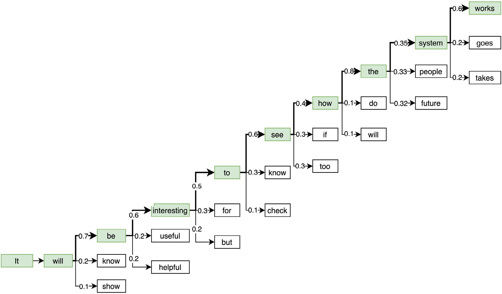
Figure 6.4 – Greedy search
As we can see, at each step, the word with the highest probability is picked up by the model under the greedy search strategy of text generation. Note the penultimate step, where the model predicts the words system, people, and future with roughly equal probabilities. With greedy search, system is selected as the next word due to it having a slightly higher probability than the rest. However, you could argue that people or future could have led to a better or more meaningful generated text.
This is the core limitation of the greedy search approach. Besides, greedy search also results in repetitive results due to a lack of randomness. If someone wants to use such a text generator artistically, greedy search is not the best approach, merely due to its monotonicity.
In the previous section, we manually wrote the text generation loop. Thanks to the transformers library, we can write the text generation step in three lines of code:
ip_ids = tkz.encode(cue, return_tensors='pt')
op_greedy = mdl.generate(ip_ids, max_length=ln)
seq = tkz.decode(op_greedy[0], skip_special_tokens=True)
print(seq)
This should output the following:
Figure 6.5 – GPT-2 generated text (concise)
Notice that the generated sentence shown in Figure 6.5 has one word less than the sentence that was generated in Figure 6.3. This difference is because in the latter code, the max_length argument includes the cue words. So, if we have one cue word, nine new words would be predicted. If we have two cue words, eight new words would be predicted (as is the case here), and so on.
Beam search
Greedy search is not the only way of generating texts. Beam search is a development of the greedy search method wherein we maintain a list of potential candidate sequences based on the overall predicted sequence probability, rather than just the next word probability. The number of candidate sequences to be pursued is the number of beams along the tree of word predictions.
The following diagram demonstrates how beam search with a beam size of three would be used to produce three candidate sequences (ordered as per the overall sequence probability) of five words each:
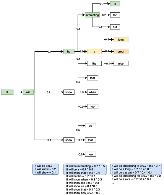
Figure 6.6 – Beam search
At each iteration in this beam search example, the three most likely candidate sequences are maintained. As we proceed further in the sequence, the possible number of candidate sequences increases exponentially. However, we are only interested in the top three sequences. This way, we do not miss potentially better sequences as we might with greedy search.
In PyTorch, we can use beam search out of the box in one line of code. The following code demonstrates beam search-based text generation with three beams generating the three most likely sentences, each containing five words:
op_beam = mdl.generate(
ip_ids,
max_length=5,
num_beams=3,
num_return_sequences=3,
)
for op_beam_cur in op_beam:
print(tkz.decode(op_beam_cur, skip_special_tokens=True))
This gives us the following output:

Figure 6.7 – Beam search results
The problem of repetitiveness or monotonicity still remains with the beam search. Different runs would result in the same set of results as it deterministically looks for the sequence with the maximum overall probabilities. In the next section, we will look at some of the ways we can make the generated text more unpredictable or creative.
Top-k and top-p sampling
Instead of always picking the next word with the highest probability, we can randomly sample the next word out of the possible set of next words based on their relative probabilities. For example, in Figure 6.6, the words be, know, and show have probabilities of 0.7, 0.2, and 0.1, respectively. Instead of always picking be against know and show, we can randomly sample any one of these three words based on their probabilities. If we repeat this exercise 10 times to generate 10 separate texts, be will be chosen roughly seven times and know and show will be chosen two and one times, respectively. This gives us far too many different possible combinations of words that beam or greedy search would never generate.
Two of the most popular ways of generating texts using sampling techniques are known as top-k and top-p sampling. Under top-k sampling, we predefine a parameter, k, which is the number of candidate words that should be considered while sampling the next word. All the other words are discarded, and the probabilities are normalized among the top k words. In our previous example, if k is 2, then the word show will be discarded and the words be and know will have their probabilities (0.7 and 0.2, respectively) normalized to 0.78 and 0.22, respectively.
The following code demonstrates the top-k text generation method:
for i in range(3):
torch.manual_seed(i)
op = mdl.generate(
ip_ids,
do_sample=True,
max_length=5,
top_k=2
)
seq = tkz.decode(op[0], skip_special_tokens=True)
print(seq)
This should generate the following output:

Figure 6.8 – Top-k search results
To sample from all possible words, instead of just the top-k words, we shall set the top-k argument to 0 in our code. As shown in the preceding screenshot, different runs produce different results as opposed to greedy search, which would result in the exact same result on each run, as shown in the following screenshot:

Figure 6.9 – Repetitive greedy search results
Under the top-p sampling strategy, instead of defining the top k words to look at, we can define a cumulative probability threshold (p) and then retain words whose probabilities add up to p. In our example, if p is between 0.7 and 0.9, then we discard know and show, if p is between 0.9 and 1.0, then we discard show, and if p is 1.0, then we keep all three words; that is, be, know, and show.
The top-k strategy can sometimes be unfair in scenarios where the probability distribution is flat. This is because it clips off words that are almost as probable as the ones that have been retained. In those cases, the top-p strategy would retain a larger pool of words to sample from and would retain a smaller pool of words in cases where the probability distribution is rather sharp.
The following code demonstrates the top-p sampling method:
for i in range(3):
torch.manual_seed(i)
op = mdl.generate(
ip_ids,
do_sample=True,
max_length=5,
top_p=0.75,
top_k=0
)
seq = tkz.decode(op[0], skip_special_tokens=True)
print(seq)
This should output the following:

Figure 6.10 – Top-p search results
We can set both top-k and top-p strategies together. In this example, we have set top-k to 0 to essentially disable the top-k strategy, and p is set to 0.75. Once again, this results in different sentences across runs and can lead us to more creatively generated texts as opposed to greedy or beam search. There are many more text generation strategies available, and a lot of research is happening in this area. We encourage you to follow up on this further.
A great starting point is playing around with the available text generation strategies in the transformers library. You can read more about it by going to this illustrative blog post from the makers of this library: https://huggingface.co/blog/how-to-generate.
This concludes our exploration of using PyTorch to generate text. In the next section, we will perform a similar exercise but this time for music instead of text. The idea is to train an unsupervised model on a music dataset and use the trained model to generate melodies similar to those in the training dataset.
Generating MIDI music with LSTMs using PyTorch
Moving on from text, in this section, we will use PyTorch to create a machine learning model that can compose classical-like music. We used transformers for generating text in the previous section. Here, we will use an LSTM model to process sequential music data. We will train the model on Mozart's classical music compositions.
Each musical piece will essentially be broken down into a sequence of piano notes. We will be reading music data in the form of Musical Instruments Digital Interface (MIDI) files, which is a well-known and commonly used format for conveniently reading and writing musical data across devices and environments.
After converting the MIDI files into sequences of piano notes (which we call the piano roll), we will use them to train a next-piano-note detection system. In this system, we will build an LSTM-based classifier that will predict the next piano note for the given preceding sequence of piano notes, of which there are 88 in total (as per the standard 88 piano keys).
We will now demonstrate the entire process of building the AI music composer in the form of an exercise. Our focus will be on the PyTorch code that's used for data loading, model training, and generating music samples. Please note that the model training process may take several hours and therefore it is recommended to run the training process in the background; for example, overnight. The code presented here has been curtailed in the interest of keeping the text short.
Details of handling the MIDI music files are beyond the scope of this book, although you are encouraged to explore the full code, which is available at https://github.com/PacktPublishing/Mastering-PyTorch/blob/master/Chapter06/music_generation.ipynb.
Loading the MIDI music data
First, we will demonstrate how to load the music data that is available in MIDI format. We will briefly mention the code for handling MIDI data, and then illustrate how to make PyTorch dataloaders out of it. Let's get started:
- As always, we will begin by importing the important libraries. Some of the new ones we'll be using in this exercise are as follows:
import skimage.io as io
from struct import pack, unpack
from io import StringIO, BytesIO
skimage is used to visualize the sequences of the music samples that are generated by the model. struct and io are used for handling the process of converting MIDI music data into piano rolls.
- Next, we will write the helper classes and functions for loading MIDI files and converting them into sequences of piano notes (matrices) that can be fed to the LSTM model. First, we define some MIDI constants in order to configure various music controls such as pitch, channels, start of sequence, end of sequence, and so on:
NOTE_MIDI_OFF = 0x80
NOTE_MIDI_ON = 0x90
MIDI_PITCH_BND = 0xE0
...
- Then, we will define a series of classes that will handle MIDI data input and output streams, the MIDI data parser, and so on, as follows:
class MOStrm:
# MIDI Output Stream
...
class MIFl:
# MIDI Input File Reader
...
class MOFl(MOStrm):
# MIDI Output File Writer
...
class RIStrFl:
# Raw Input Stream File Reader
...
class ROStrFl:
# Raw Output Stream File Writer
...
class MFlPrsr:
# MIDI File Parser
...
class EvtDspch:
# Event Dispatcher
...
# MIDI Data Reader
...
- Having handled all the MIDI data I/O-related code, we are all set to instantiate our own PyTorch dataset class. Before we do that, we must define two crucial functions – one for converting the read MIDI file into a piano roll and one for padding the piano roll with empty notes. This will normalize the lengths of the musical pieces across the dataset:
def md_fl_to_pio_rl(md_fl):
md_d = MidiDataRead(md_fl, dtm=0.3)
pio_rl = md_d.pio_rl.transpose()
pio_rl[pio_rl > 0] = 1
return pio_rl
def pd_pio_rl(pio_rl, mx_l=132333, pd_v=0):
orig_rol_len = pio_rl.shape[1]
pdd_rol = np.zeros((88, mx_l))
pdd_rol[:] = pd_v
pdd_rol[:, - orig_rol_len:] = pio_rl
return pdd_rol
- Now, we can define our PyTorch dataset class, as follows:
class NtGenDataset(data.Dataset):
def __init__(self, md_pth, mx_seq_ln=1491):
...
def mx_len_upd(self):
...
def __len__(self):
return len(self.md_fnames_ful)
def __getitem__(self, index):
md_fname_ful = self.md_fnames_ful[index]
pio_rl = md_fl_to_pio_rl(md_fname_ful)
seq_len = pio_rl.shape[1] - 1
ip_seq = pio_rl[:, :-1]
gt_seq = pio_rl[:, 1:]
...
return (torch.FloatTensor(ip_seq_pad),
torch.LongTensor(gt_seq_pad), torch.LongTensor([seq_len]))
- Besides the dataset class, we must add another helper function to post-process the music sequences in a batch of training data into three separate lists. These will be input sequences, output sequences, and lengths of sequences, ordered by the lengths of the sequences in descending order:
def pos_proc_seq(btch):
ip_seqs, op_seqs, lens = btch
...
ord_tr_data_tups = sorted(tr_data_tups,
key=lambda c: int(c[2]),
reverse=True)
ip_seq_splt_btch, op_seq_splt_btch, btch_splt_lens = zip(*ord_tr_data_tups)
...
return tps_ip_seq_btch, ord_op_seq_btch, list(ord_btch_lens_l)
- For this exercise, we will be using a set of Mozart's compositions. You can download the dataset from here: http://www.piano-midi.de/mozart.htm . The downloaded folder consists of 21 MIDI files, which we will split into 18 training and three validation set files. The downloaded data is stored under ./mozart/train and ./mozart/valid. Once downloaded, we can read the data and instantiate our own training and validation dataset loaders:
training_dataset = NtGenDataset('./mozart/train', mx_seq_ln=None)
training_datasetloader = data.DataLoader(training_dataset, batch_size=5,shuffle=True, drop_last=True)
validation_dataset = NtGenDataset('./mozart/valid/', mx_seq_ln=None)
validation_datasetloader = data.DataLoader(validation_dataset, batch_size=3, shuffle=False, drop_last=False)
X_validation = next(iter(validation_datasetloader))
X_validation[0].shape
This should give us the following output:
Figure 6.11 – Sample music data dimensions
As we can see, the first validation batch consists of three sequences of length 1,587 (notes), where each sequence is encoded into an 88-size vector, with 88 being the total number of piano keys. For those of you who are trained musicians, here is a music sheet equivalent of the first few notes of one of the validation set music files:
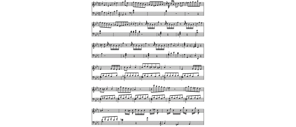
Figure 6.12 – Music sheet of a Mozart composition
Alternatively, we can visualize the sequence of notes as a matrix with 88 rows, one per piano key. The following is a visual matrix representation of the preceding melody (the first 300 notes out of 1,587):

Figure 6.13 – Matrix representation of a Mozart composition
Dataset citation
The MIDI, audio (MP3, OGG), and video files of Bernd Krueger are licensed under the CC BY-SA Germany License.Name: Bernd Krueger Source: http://www.piano-midi.de The distribution or public playback of these files is only allowed under identical license conditions.The scores are open source.
We will now define the LSTM model and training routine.
Defining the LSTM model and training routine
So far, we have managed to successfully load a MIDI dataset and use it to create our own training and validation data loaders. In this section, we will define the LSTM model architecture, as well as the training and evaluation routines that shall be run during the model training loop. Let's get started:
- First, we must define the model architecture. As we mentioned earlier, we will use an LSTM model that consists of an encoder layer that encodes the 88-dimensional representation of the input data at each time step of the sequence into a 512-dimensional hidden layer representation. The encoder is followed by two LSTM layers, followed by a fully connected layer that finally softmaxes into the 88 classes.
As per the different types of recurrent neural networks (RNNs) we discussed in Chapter 4, Deep Recurrent Model Architectures, this is a many-to-one sequence classification task, where the input is the entire sequence from time step 0 to time step t and the output is one of the 88 classes at time step t+1, as follows:
class MusicLSTM(nn.Module):
def __init__(self, ip_sz, hd_sz, n_cls, lyrs=2):
...
self.nts_enc = nn.Linear(in_features=ip_sz, out_features=hd_sz)
self.bn_layer = nn.BatchNorm1d(hd_sz)
self.lstm_layer = nn.LSTM(hd_sz, hd_sz, lyrs)
self.fc_layer = nn.Linear(hd_sz, n_cls)
def forward(self, ip_seqs, ip_seqs_len, hd=None):
...
pkd = torch.nn.utils.rnn.pack_padded_sequence(nts_enc_ful, ip_seqs_len)
op, hd = self.lstm_layer(pkd, hd)
...
lgts = self.fc_layer(op_nrm_drp.permute(2,0,1))
...
zero_one_lgts = torch.stack((lgts, rev_lgts), dim=3).contiguous()
flt_lgts = zero_one_lgts.view(-1, 2)
return flt_lgts, hd
- Once the model architecture has been defined, we can specify the model training routine. We will use the Adam optimizer with gradient clipping to avoid overfitting. Another measure that's already in place to counter overfitting is the use of a dropout layer, as specified in the previous step:
def lstm_model_training(lstm_model, lr, ep=10, val_loss_best=float("inf")):
...
for curr_ep in range(ep):
...
for batch in training_datasetloader:
...
lgts, _ = lstm_model(ip_seq_b_v, seq_l)
loss = loss_func(lgts, op_seq_b_v)
...
if vl_ep_cur < val_loss_best:
torch.save(lstm_model.state_dict(), 'best_model.pth')
val_loss_best = vl_ep_cur
return val_loss_best, lstm_model
- Similarly, we will define the model evaluation routine, where a forward pass is run on the model with its parameters remaining unchanged:
def evaluate_model(lstm_model):
...
for batch in validation_datasetloader:
...
lgts, _ = lstm_model(ip_seq_b_v, seq_l)
loss = loss_func(lgts, op_seq_b_v)
vl_loss_full += loss.item()
seq_len += sum(seq_l)
return vl_loss_full/(seq_len*88)
Now, let's train and test the music generation model.
Training and testing the music generation model
In this final section, we will actually train the LSTM model. We will then use the trained music generation model to generate a music sample that we can listen to and analyze. Let's get started:
- We are all set to instantiate our model and start training it. We have used categorical cross-entropy as the loss function for this classification task. We are training the model with a learning rate of 0.01 for 10 epochs:
loss_func = nn.CrossEntropyLoss().cpu()
lstm_model = MusicLSTM(ip_sz=88, hd_sz=512, n_cls=88).cpu()
val_loss_best, lstm_model = lstm_model_training(lstm_model, lr=0.01, ep=10)
This should output the following:

- Here comes the fun part. Once we have a next-musical-note-predictor, we can use it as a music generator. All we need to do is simply initiate the prediction process by providing an initial note as a cue. The model can then recursively make predictions for the next note at each time step, wherein the predictions at time step t are appended to the input sequence at time t+1.
Here, we will write a music generation function that takes in the trained model object, the intended length of music to be generated, a starting note to the sequence, and temperature. Temperature is a standard mathematical operation over the softmax function at the classification layer. It is used to manipulate the distribution of softmax probabilities, either by broadening or shrinking the softmaxed probabilities distribution. The code is as follows:
def generate_music(lstm_model, ln=100, tmp=1, seq_st=None):
...
for i in range(ln):
op, hd = lstm_model(seq_ip_cur, [1], hd)
probs = nn.functional.softmax(op.div(tmp), dim=1)
...
gen_seq = torch.cat(op_seq, dim=0).cpu().numpy()
return gen_seq
Finally, we can use this function to create a brand-new music composition:
seq = generate_music(lstm_model, ln=100, tmp=1, seq_st=None)
midiwrite('generated_music.mid', seq, dtm=0.2)
This should create the musical piece and save it as a MIDI file in the current directory. We can open the file and play it to hear what the model has produced. Nonetheless, we can also view the visual matrix representation of the produced music:

Figure 6.15 – Matrix representation of an AI generated music sample
Furthermore, here is what the generated music would look like as a music sheet:
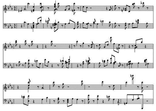
Figure 6.16 – Music sheet of an AI generated music sample
Here, we can see that the generated melody seems to be not quite as melodious as Mozart's original compositions. Nonetheless, you can see consistencies in some key combinations that the model has learned. Moreover, the generated music quality can be enhanced by training the model on more data, as well as training it for more epochs.
This concludes our exercise on using machine learning to generate music. In this section, we have demonstrated how to use existing musical data to train a note predictor model from scratch and use the trained model to generate music. In fact, you can extend the idea of using generative models to generate samples of any kind of data. PyTorch is an extremely effective tool when it comes to such use cases, especially due to its straightforward APIs for data loading, model building/training/testing, and using trained models as data generators. You are encouraged to try out more such tasks on different use cases and data types.
Summary
In this chapter, we explored generative models using PyTorch. Beginning with text generation, we utilized the transformer-based language model we built in the previous chapter to develop a text generator. We demonstrated how PyTorch can be used to convert a model that's been trained without supervision (a language model, in this case) into a data generator. After that, we exploited the pre-trained advanced transformer models that are available under the transformers library and used them as text generators. We discussed various text generation strategies, such as greedy search, beam search, and top-k and top-p sampling.
Next, we built an AI music composer from scratch. Using Mozart's piano compositions, we trained an LSTM model to predict the next piano note given by the preceding sequence of piano notes. After that, we used the classifier we trained without supervision as a data generator to create music. The results of both the text and the music generators are promising and show how powerful PyTorch can be as a resource for developing artistic AI generative models.
In the same artistic vein, in the next chapter, we shall learn how machine learning can be used to transfer the style of one image to another. With PyTorch at our disposal, we will use CNNs to learn artistic styles from various images and impose those styles on different images – a task better known as neural style transfer.