Chapter 3: Deep CNN Architectures
In this chapter, we will first briefly review the evolution of CNNs (in terms of architectures), and then we will study the different CNN architectures in detail. We will implement these CNN architectures using PyTorch and in doing so, we aim to exhaustively explore the tools (modules and built-in functions) that PyTorch has to offer in the context of building Deep CNNs. Building strong CNN expertise in PyTorch will enable us to solve a number of deep learning problems involving CNNs. This will also help us in building more complex deep learning models or applications of which CNNs are a part.
This chapter will cover the following topics:
- Why are CNNs so powerful?
- Evolution of CNN architectures
- Developing LeNet from scratch
- Fine-tuning the AlexNet model
- Running a pre-trained VGG model
- Exploring GoogLeNet and Inception v3
- Discussing ResNet and DenseNet architectures
- Understanding EfficientNets and the future of CNN architectures
Technical requirements
We will be using Jupyter Notebooks for all of our exercises. The following is the list of Python libraries that should be installed for this chapter using pip. For example, use run pip install torch==1.4.0 on the command line, and so on:
jupyter==1.0.0
torch==1.4.0
torchvision==0.5.0
nltk==3.4.5
Pillow==6.2.2
pycocotools==2.0.0
All the code files relevant to this chapter are available at https://github.com/PacktPublishing/Mastering-PyTorch/tree/master/Chapter03.
Why are CNNs so powerful?
CNNs are among the most powerful machine learning models at solving challenging problems such as image classification, object detection, object segmentation, video processing, natural language processing, and speech recognition. Their success is attributed to various factors, such as the following:
- Weight sharing: This makes CNNs parameter-efficient, that is, different features are extracted using the same set of weights or parameters. Features are the high-level representations of input data that the model generates with its parameters.
- Automatic feature extraction: Multiple feature extraction stages help a CNN to automatically learn feature representations in a dataset.
- Hierarchical learning: The multi-layered CNN structure helps CNNs to learn low-, mid-, and high-level features.
- The ability to explore both spatial and temporal correlations in the data, such as in video processing tasks.
Besides these pre-existing fundamental characteristics, CNNs have advanced over the years with the help of improvements in the following areas:
- The use of better activation and loss functions, such as using ReLU to overcome the vanishing gradient problem. What is the vanishing gradient problem? Well, we know backpropagation in neural networks works on the basis of the chain rule of differentiation.
According to the chain rule, the gradient of the loss function with respect to the input layer parameters can be written as a product of gradients at each layer. If these gradients are all less than 1 – and worse still, tending toward 0 – then the product of these gradients will be a vanishingly small value. The vanishing gradient problem can cause serious troubles in the optimization process by preventing the network parameters from changing their values, which is equivalent to stunted learning.
- Parameter optimization, such as using an optimizer based on Adaptive Momentum (Adam) instead of simple Stochastic Gradient Descent.
- Regularization: Applying dropouts and batch normalization besides L2 regularization.
But some of the most significant drivers of development in CNNs over the years have been the various architectural innovations:
- Spatial exploration-based CNNs: The idea behind spatial exploration is using different kernel sizes in order to explore different levels of visual features in input data. The following diagram shows a sample architecture for a spatial exploration-based CNN model:

Figure 3.1 – Spatial exploration-based CNN
- Depth-based CNNs: The depth here refers to the depth of the neural network, that is, the number of layers. So, the idea here is to create a CNN model with multiple convolutional layers in order to extract highly complex visual features. The following diagram shows an example of such a model architecture:

Figure 3.2 – Depth-based CNN
- Width-based CNNs: Width refers to the number of channels or feature maps in the data or features extracted from the data. So, width-based CNNs are all about increasing the number of feature maps as we go from the input to the output layers, as demonstrated in the following diagram:
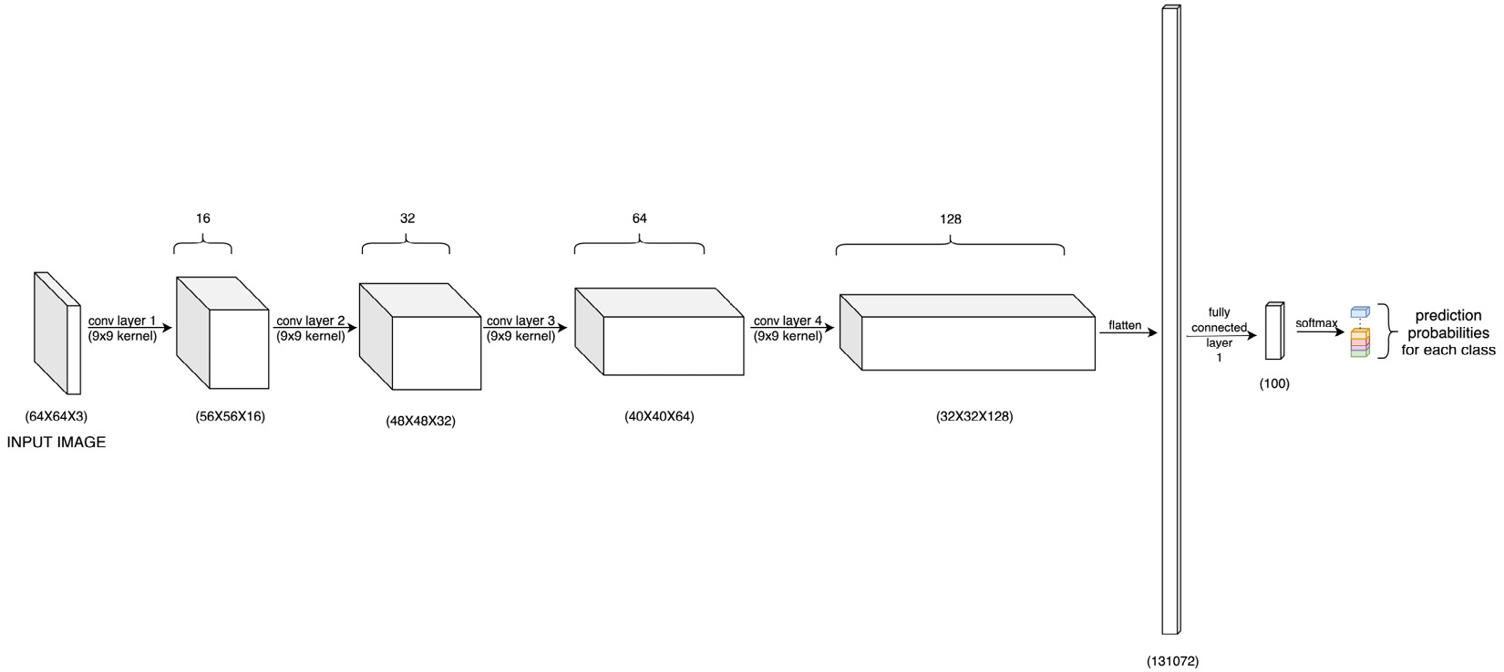
Figure 3.3 – Width-based CNN
- Multi-path-based CNNs: So far, the preceding three types of architectures have monotonicity in connections between layers, that is, direct connections exist only between consecutive layers. Multi-path CNNs brought the idea of making shortcut connections or skip connections between non-consecutive layers. The following diagram shows an example of a multi-path CNN model architecture:

Figure 3.4 – Multi-path CNN
A key advantage of multi-path architectures is a better flow of information across several layers, thanks to the skip connections. This, in turn, also lets the gradient flow back to the input layers without too much dissipation.
Having looked at the different architectural setups found in CNN models, we will now look at how CNNs have evolved over the years ever since they were first used.
Evolution of CNN architectures
CNNs have been in existence since 1989, when the first multilayered CNN, called ConvNet, was developed by Yann LeCun. This model could perform visual cognition tasks such as identifying handwritten digits. In 1998, LeCun developed an improved ConvNet model called LeNet. Due to its high accuracy in optical recognition tasks, LeNet was adopted for industrial use soon after its invention. Ever since, CNNs have been one of the most successful machine learning models, both in industry as well as academia. The following diagram shows a brief timeline of architectural developments in the lifetime of CNNs, starting from 1989 all the way to 2020:
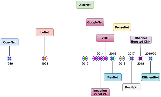
Figure 3.5 – CNN architecture evolution – a broad picture
As we can see, there is a significant gap between the years 1998 and 2012. This was primarily because there wasn't a dataset big and suitable enough to demonstrate the capabilities of CNNs, especially deep CNNs. And on the existing small datasets of the time, such as MNIST, classical machine learning models such as SVMs were starting to beat CNN performance. During those years, a few CNN developments took place.
The ReLU activation function was designed in order to deal with the gradient explosion and decay problem during backpropagation. Non-random initialization of network parameter values proved to be crucial. Max-pooling was invented as an effective method for subsampling. GPUs were getting popular for training neural networks, especially CNNs at scale. Finally, and most importantly, a large-scale dedicated dataset of annotated images called ImageNet (http://www.image-net.org/) was created by a research group at Stanford. This dataset is still one of the primary benchmarking datasets for CNN models to date.
With all of these developments compounding over the years, in 2012, a different architectural design brought about a massive improvement in CNN performance on the ImageNet dataset. This network was called AlexNet (named after the creator, Alex Krizhevsky). AlexNet, along with having various novel aspects such as random cropping and pre-training, established the trend of uniform and modular convolutional layer design. The uniform and modular layer structure was taken forward by repeatedly stacking such modules (of convolutional layers), resulting in very deep CNNs also known as VGGs.
Another approach of branching the blocks/modules of convolutional layers and stacking these branched blocks on top of each other proved extremely effective for tailored visual tasks. This network was called GoogLeNet (as it was developed at Google) or Inception v1 (inception being the term for those branched blocks). Several variants of the VGG and Inception networks followed, such as VGG16, VGG19, Inception v2, Inception v3, and so on.
The next phase of development began with skip connections. To tackle the problem of gradient decay while training CNNs, non-consecutive layers were connected via skip connections lest information dissipated between them due to small gradients. A popular type of network that emerged with this trick, among other novel characteristics such as batch normalization, was ResNet.
A logical extension of ResNet was DenseNet, where layers were densely connected to each other, that is, each layer gets the input from all the previous layers' output feature maps. Furthermore, hybrid architectures were then developed by mixing successful architectures from the past such as Inception-ResNet and ResNeXt, where the parallel branches within a block were increased in number.
Lately, the channel boosting technique has proven useful in improving CNN performance. The idea here is to learn novel features and exploit pre-learned features through transfer learning. Most recently, automatically designing new blocks and finding optimal CNN architectures has been a growing trend in CNN research. Examples of such CNNs are MnasNets and EfficientNets. The approach behind these models is to perform a neural architecture search to deduce an optimal CNN architecture with a uniform model scaling approach.
In the next section, we will go back to one of the earliest CNN models and take a closer look at the various CNN architectures developed since. We will build these architectures using PyTorch, training some of the models on real-world datasets. We will also explore PyTorch's pre-trained CNN models repository, popularly known as model-zoo. We will learn how to fine-tune these pre-trained models as well as running predictions on them.
Developing LeNet from scratch
LeNet, originally known as LeNet-5, is one of the earliest CNN models, developed in 1998. The number 5 in LeNet-5 represents the total number of layers in this model, that is, two convolutional and three fully connected layers. With roughly 60,000 total parameters, this model gave state-of-the-art performance on image recognition tasks for handwritten digit images in the year 1998. As expected from a CNN model, LeNet demonstrated rotation, position, and scale invariance as well as robustness against distortion in images. Contrary to the classical machine learning models of the time, such as SVMs, which treated each pixel of the image separately, LeNet exploited the correlation among neighboring pixels.
Note that although LeNet was developed for handwritten digit recognition, it can certainly be extended for other image classification tasks, as we shall see in our next exercise. The following diagram shows the architecture of a LeNet model:
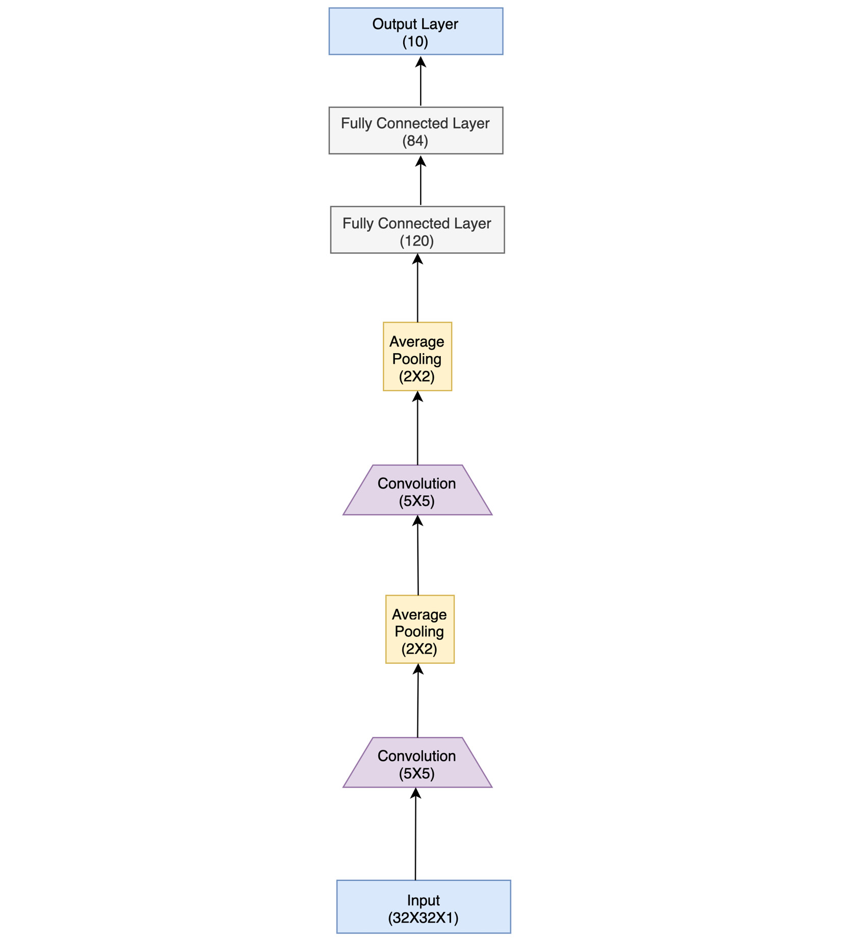
Figure 3.6 – LeNet architecture
As mentioned earlier, there are two convolutional layers followed by three fully connected layers (including the output layer). This approach of stacking convolutional layers followed by fully connected layers later became a trend in CNN research and is still applied to the latest CNN models. Besides these layers, there are pooling layers in between. These are basically subsampling layers that reduce the spatial size of image representation, thereby reducing the number of parameters and computations. The pooling layer used in LeNet was an average pooling layer that had trainable weights. Soon after, max pooling emerged as the most commonly used pooling function in CNNs.
The numbers in brackets in each layer in the figure demonstrate the dimensions (for input, output, and fully connected layers) or window size (for convolutional and pooling layers). The expected input for a grayscale image is 32x32 pixels in size. This image is then operated on by 5x5 convolutional kernels, followed by 2x2 pooling, and so on. The output layer size is 10, representing the 10 classes.
In this section, we will use PyTorch to build LeNet from scratch and train and evaluate it on a dataset of images for the task of image classification. We will see how easy and intuitive it is to build the network architecture in PyTorch using the outline from Figure 3.6.
Furthermore, we will demonstrate how effective LeNet is, even on a dataset different from the ones it was originally developed on (that is, MNIST) and how PyTorch makes it easy to train and test the model in a few lines of code.
Using PyTorch to build LeNet
Observe the following steps to build the model:
- For this exercise, we will need to import a few dependencies. Execute the following import statements:
import numpy as np
import matplotlib.pyplot as plt
import torch
import torchvision
import torch.nn as nn
import torch.nn.functional as F
import torchvision.transforms as transforms
torch.manual_seed(55)
Here, we are importing all the torch modules necessary for the exercise. We also import numpy and matplotlib to display images during the exercise. Besides imports, we also set the random seed to ensure the reproducibility of this exercise.
- Next, we will define the model architecture based on the outline given in Figure 3.6:
class LeNet(nn.Module):
def __init__(self):
super(LeNet, self).__init__()
# 3 input image channel, 6 output feature maps and 5x5 conv kernel
self.cn1 = nn.Conv2d(3, 6, 5)
# 6 input image channel, 16 output feature maps and 5x5 conv kernel
self.cn2 = nn.Conv2d(6, 16, 5)
# fully connected layers of size 120, 84 and 10
self.fc1 = nn.Linear(16 * 5 * 5, 120) # 5*5 is the spatial dimension at this layer
self.fc2 = nn.Linear(120, 84)
self.fc3 = nn.Linear(84, 10)
def forward(self, x):
# Convolution with 5x5 kernel
x = F.relu(self.cn1(x))
# Max pooling over a (2, 2) window
x = F.max_pool2d(x, (2, 2))
# Convolution with 5x5 kernel
x = F.relu(self.cn2(x))
# Max pooling over a (2, 2) window
x = F.max_pool2d(x, (2, 2))
# Flatten spatial and depth dimensions into a single vector
x = x.view(-1, self.flattened_features(x))
# Fully connected operations
x = F.relu(self.fc1(x))
x = F.relu(self.fc2(x))
x = self.fc3(x)
return x
def flattened_features(self, x):
# all except the first (batch) dimension
size = x.size()[1:]
num_feats = 1
for s in size:
num_feats *= s
return num_feats
lenet = LeNet()
print(lenet)
In the last two lines, we instantiate the model and print the network architecture. The output will be as follows:
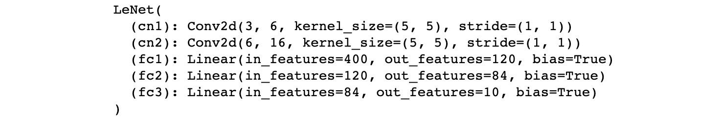
Figure 3.7 – LeNet PyTorch model object
There are the usual __init__ and forward methods for architecture definition and running a forward pass, respectively. The additional flattened_features method is meant to calculate the total number of features in an image representation layer (usually an output of a convolutional layer or pooling layer). This method helps to flatten the spatial representation of features into a single vector of numbers, which is then used as input to fully connected layers.
Besides the details of the architecture mentioned earlier, ReLU is used throughout the network as the activation function. Also, contrary to the original LeNet network, which takes in single-channel images, the current model is modified to accept RGB images, that is, three channels as input. This is done in order to adapt to the dataset that is used for this exercise.
- We then define the training routine, that is, the actual backpropagation step:
def train(net, trainloader, optim, epoch):
# initialize loss
loss_total = 0.0
for i, data in enumerate(trainloader, 0):
# get the inputs; data is a list of [inputs, labels]
# ip refers to the input images, and ground_truth refers to the output classes the images belong to
ip, ground_truth = data
# zero the parameter gradients
optim.zero_grad()
# forward-pass + backward-pass + optimization -step
op = net(ip)
loss = nn.CrossEntropyLoss()(op, ground_truth)
loss.backward()
optim.step()
# update loss
loss_total += loss.item()
# print loss statistics
if (i+1) % 1000 == 0: # print at the interval of 1000 mini-batches
print('[Epoch number : %d, Mini-batches: %5d] loss: %.3f' % (epoch + 1, i + 1, loss_total / 200))
loss_total = 0.0
For each epoch, this function iterates through the entire training dataset, runs a forward pass through the network and, using backpropagation, updates the parameters of the model based on the specified optimizer. After iterating through every 1,000 mini-batches of the training dataset, this method also logs the calculated loss.
- Similar to the training routine, we will define the test routine that we will use to evaluate model performance:
def test(net, testloader):
success = 0
counter = 0
with torch.no_grad():
for data in testloader:
im, ground_truth = data
op = net(im)
_, pred = torch.max(op.data, 1)
counter += ground_truth.size(0)
success += (pred == ground_truth).sum().item()
print('LeNet accuracy on 10000 images from test dataset: %d %%' % (100 * success / counter))
This function runs a forward pass through the model for each test-set image, calculates the correct number of predictions, and prints the percentage of correct predictions on the test set.
- Before we get on to training the model, we need to load the dataset. For this exercise, we will be using the CIFAR-10 dataset.
Dataset citation
Learning Multiple Layers of Features from Tiny Images, Alex Krizhevsky, 2009
This dataset consists of 60,000 32x32 RGB images labeled across 10 classes, with 6,000 images per class. The 60,000 images are split into 50,000 training images and 10,000 test images. More details can be found here: https://www.cs.toronto.edu/~kriz/cifar.html. Torch supports the CIFAR dataset under the torchvision.datasets module. We will be using the module to directly load the data and instantiate train and test dataloaders as demonstrated in the following code:
# The mean and std are kept as 0.5 for normalizing pixel values as the pixel values are originally in the range 0 to 1
train_transform = transforms.Compose([transforms.RandomHorizontalFlip(),
transforms.RandomCrop(32, 4),
transforms.ToTensor(),
transforms.Normalize((0.5, 0.5, 0.5), (0.5, 0.5, 0.5))])
trainset = torchvision.datasets.CIFAR10(root='./data', train=True, download=True, transform=train_transform)
trainloader = torch.utils.data.DataLoader(trainset, batch_size=8, shuffle=True, num_workers=1)
test_transform = transforms.Compose([transforms.ToTensor(), transforms.Normalize((0.5, 0.5, 0.5), (0.5, 0.5, 0.5))])
testset = torchvision.datasets.CIFAR10(root='./data', train=False, download=True, transform=test_transform)
testloader = torch.utils.data.DataLoader(testset, batch_size=10000, shuffle=False, num_workers=2)
# ordering is important
classes = ('plane', 'car', 'bird', 'cat', 'deer', 'dog', 'frog', 'horse', 'ship', 'truck')
Note
In the previous chapter, we manually downloaded the dataset and wrote a custom dataset class and a dataloader function. We will not need to write those here, thanks to the torchvision.datasets module.
Because we set the download flag to True, the dataset will be downloaded locally. Then, we shall see the following dialog box:

Figure 3.8 – CIFAR-10 dataset download
The transformations used for training and testing datasets are different because we apply some data augmentation to the training dataset, such as flipping and cropping, which are not applicable to the test dataset. Also, after defining trainloader and testloader, we declare the 10 classes in this dataset with a pre-defined ordering.
- After loading the datasets, let's investigate how the data looks:
# define a function that displays an image
def imageshow(image):
# un-normalize the image
image = image/2 + 0.5
npimage = image.numpy()
plt.imshow(np.transpose(npimage, (1, 2, 0)))
plt.show()
# sample images from training set
dataiter = iter(trainloader)
images, labels = dataiter.next()
# display images in a grid
num_images = 4
imageshow(torchvision.utils.make_grid(images[:num_images]))
# print labels
print(' '+' || '.join(classes[labels[j]] for j in range(num_images)))
The preceding code shows us four sample images with their respective labels from the training dataset. The output will be as follows:
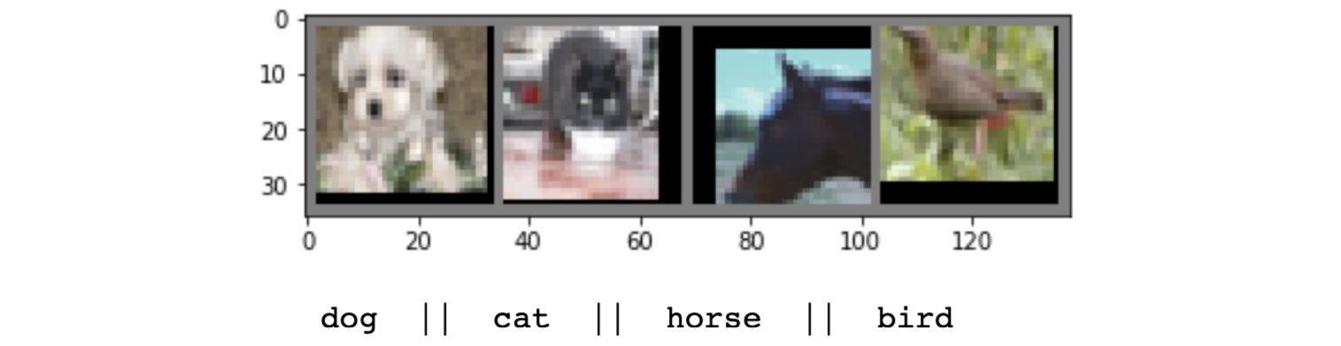
Figure 3.9 – CIFAR-10 dataset samples
The preceding output shows us four color images, which are 32x32 pixels in size. These four images belong to four different labels, as displayed in the text following the images.
We will now train the LeNet model.
Training LeNet
Now we are ready to train the model. Let's do so with the help of the following steps:
- We will define optimizer and start the training loop as shown here:
# define optimizer
optim = torch.optim.Adam(lenet.parameters(), lr=0.001)
# training loop over the dataset multiple times
for epoch in range(50):
train(lenet, trainloader, optim, epoch)
print()
test(lenet, testloader)
print()
print('Finished Training')
The output will be as follows:
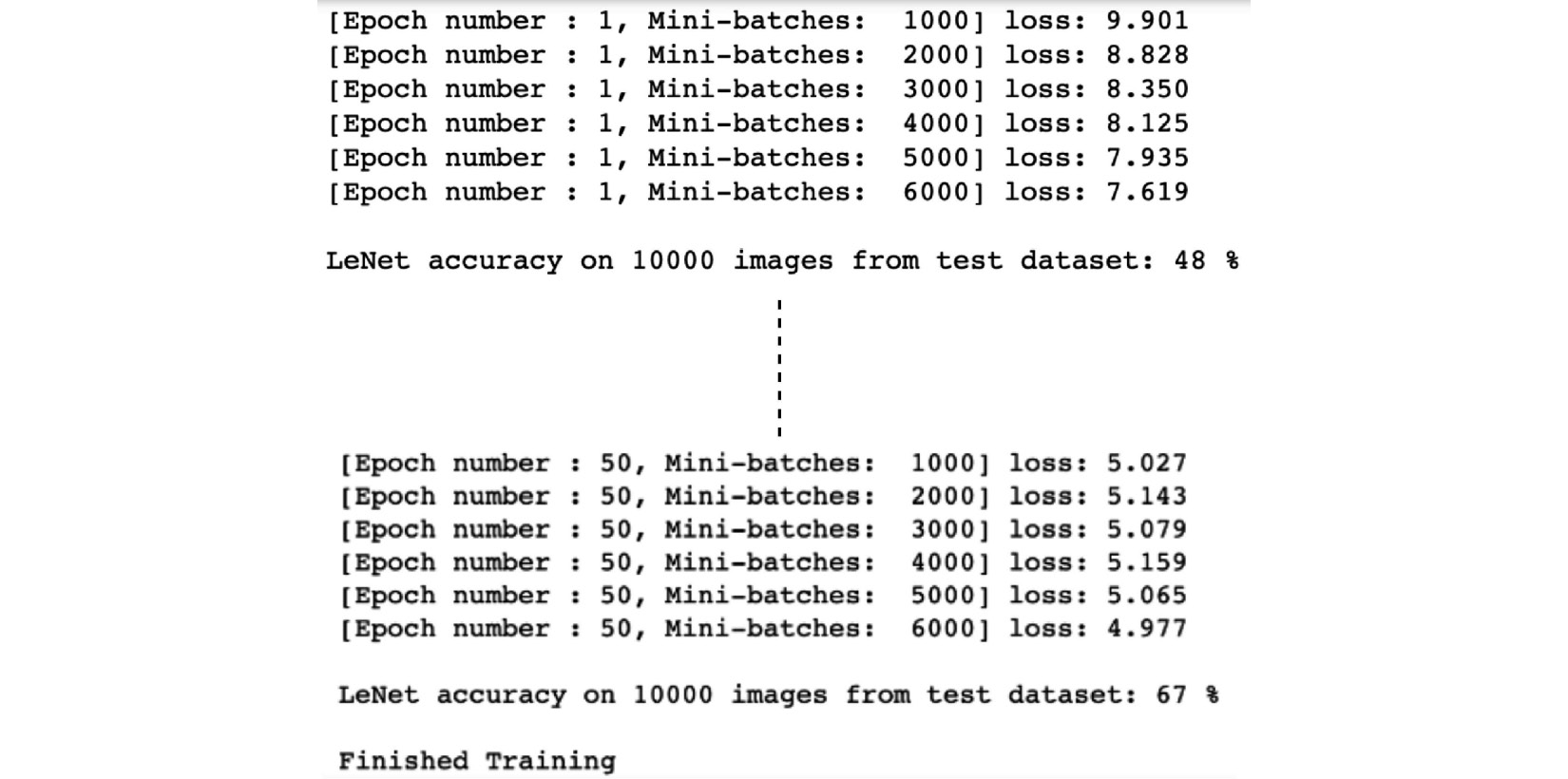
Figure 3.10 – Training LeNet
- Once the training is finished, we can save the model file locally:
model_path = './cifar_model.pth'
torch.save(lenet.state_dict(), model_path)
Having trained the LeNet model, we will now test its performance on the test dataset in the next section.
Testing LeNet
The following steps need to be observed to test the LeNet model:
- Let's make predictions by loading the saved model and running it on the test dataset:
# load test dataset images
d_iter = iter(testloader)
im, ground_truth = d_iter.next()
# print images and ground truth
imageshow(torchvision.utils.make_grid(im[:4]))
print('Label: ', ' '.join('%5s' % classes[ground_truth[j]] for j in range(4)))
# load model
lenet_cached = LeNet()
lenet_cached.load_state_dict(torch.load(model_path))
# model inference
op = lenet_cached(im)
# print predictions
_, pred = torch.max(op, 1)
print('Prediction: ', ' '.join('%5s' % classes[pred[j]] for j in range(4)))
The output will be as follows:
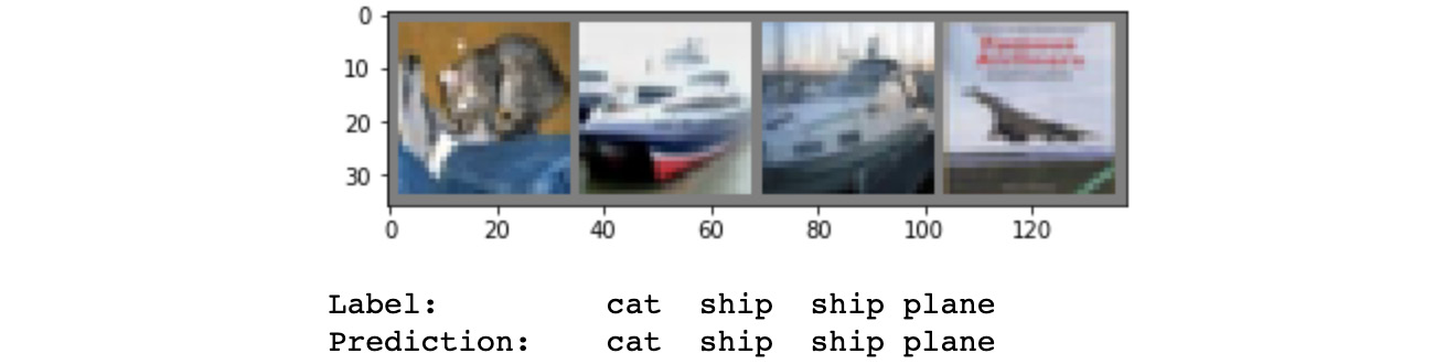
Figure 3.11 – LeNet predictions
Evidently, all four predictions are correct.
- Finally, we will check the overall accuracy of this model on the test dataset as well as per class accuracy:
success = 0
counter = 0
with torch.no_grad():
for data in testloader:
im, ground_truth = data
op = lenet_cached(im)
_, pred = torch.max(op.data, 1)
counter += ground_truth.size(0)
success += (pred == ground_truth).sum().item()
print('Model accuracy on 10000 images from test dataset: %d %%' % (
100 * success / counter))
The output will be as follows:

Figure 3.12 – LeNet overall accuracy
- For per class accuracy, the code is as follows:
class_sucess = list(0. for i in range(10))
class_counter = list(0. for i in range(10))
with torch.no_grad():
for data in testloader:
im, ground_truth = data
op = lenet_cached(im)
_, pred = torch.max(op, 1)
c = (pred == ground_truth).squeeze()
for i in range(10000):
ground_truth_curr = ground_truth[i]
class_sucess[ground_truth_curr] += c[i].item()
class_counter[ground_truth_curr] += 1
for i in range(10):
print('Model accuracy for class %5s : %2d %%' % (
classes[i], 100 * class_sucess[i] / class_counter[i]))
The output will be as follows:

Figure 3.13 – LeNet per class accuracy
Some classes have better performance than others. Overall, the model is far from perfect (that is, 100% accuracy) but much better than a model making random predictions, which would have an accuracy of 10% (due to the 10 classes).
Having built a LeNet model from scratch and evaluated its performance using PyTorch, we will now move on to a successor of LeNet – AlexNet. For LeNet, we built the model from scratch, trained, and tested it. For AlexNet, we will use a pre-trained model, fine-tune it on a smaller dataset, and test it.
Fine-tuning the AlexNet model
In this section, we will first take a quick look at the AlexNet architecture and how to build one by using PyTorch. Then we will explore PyTorch's pre-trained CNN models repository, and finally, use a pre-trained AlexNet model for fine-tuning on an image classification task, as well as making predictions.
AlexNet is a successor of LeNet with incremental changes in the architecture, such as 8 layers (5 convolutional and 3 fully connected) instead of 5, and 60 million model parameters instead of 60,000, as well as using MaxPool instead of AvgPool. Moreover, AlexNet was trained and tested on a much bigger dataset – ImageNet, which is over 100 GB in size, as opposed to the MNIST dataset (on which LeNet was trained), which amounts to a few MBs. AlexNet truly revolutionized CNNs as it emerged as a significantly more powerful class of models on image-related tasks than the other classical machine learning models, such as SVMs. Figure 3.14 shows the AlexNet architecture:
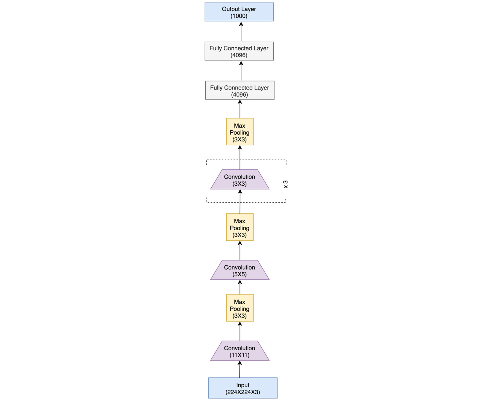
Figure 3.14 – AlexNet architecture
As we can see, the architecture follows the common theme from LeNet of having convolutional layers stacked sequentially, followed by a series of fully connected layers toward the output end. PyTorch makes it easy to translate such a model architecture into actual code. This can be seen in the following PyTorch code equivalent of the architecture:
class AlexNet(nn.Module):
def __init__(self, number_of_classes):
super(AlexNet, self).__init__()
self.feats = nn.Sequential(
nn.Conv2d(in_channels=3, out_channels=64, kernel_size=11, stride=4, padding=5),
nn.ReLU(),
nn.MaxPool2d(kernel_size=2, stride=2),
nn.Conv2d(in_channels=64, out_channels=192, kernel_size=5, padding=2),
nn.ReLU(),
nn.MaxPool2d(kernel_size=2, stride=2),
nn.Conv2d(in_channels=192, out_channels=384, kernel_size=3, padding=1),
nn.ReLU(),
nn.Conv2d(in_channels=384, out_channels=256, kernel_size=3, padding=1),
nn.ReLU(),
nn.Conv2d(in_channels=256, out_channels=256, kernel_size=3, padding=1),
nn.ReLU(),
nn.MaxPool2d(kernel_size=2, stride=2),
)
self.clf = nn.Linear(in_features=256, out_features=number_of_classes)
def forward(self, inp):
op = self.feats(inp)
op = op.view(op.size(0), -1)
op = self.clf(op)
return op
The code is quite self-explanatory, wherein the __init__ function contains the initialization of the whole layered structure, consisting of convolutional, pooling, and fully connected layers, along with ReLU activations. The forward function simply runs a data point x through this initialized network. Please note that the second line of the forward method already performs the flattening operation so that we need not define that function separately as we did for LeNet.
But besides the option of initializing the model architecture and training it ourselves, PyTorch, with its torchvision package, provides a models sub-package, which contains definitions of CNN models meant for solving different tasks, such as image classification, semantic segmentation, object detection, and so on. Following is a list of available models for the task of image classification (source: https://pytorch.org/docs/stable/torchvision/models.html):
- AlexNet
- VGG
- ResNet
- SqueezeNet
- DenseNet
- Inception v3
- GoogLeNet
- ShuffleNet v2
- MobileNet v2
- ResNeXt
- Wide ResNet
- MNASNet
In the next section, we will use a pre-trained AlexNet model as an example and demonstrate how to fine-tune it using PyTorch in the form of an exercise.
Using PyTorch to fine-tune AlexNet
In the following exercise, we will load a pre-trained AlexNet model and fine-tune it on an image classification dataset different from ImageNet (on which it was originally trained). Finally, we will test the fine-tuned model's performance to see if it could transfer-learn from the new dataset. Some parts of the code in the exercise are trimmed for readability but you can find the full code here: https://github.com/PacktPublishing/Mastering-PyTorch/blob/master/Chapter03/transfer_learning_alexnet.ipynb.
For this exercise, we will need to import a few dependencies. Execute the following import statements:
import os
import time
import copy
import numpy as np
import matplotlib.pyplot as plt
import torch
import torchvision
import torch.nn as nn
import torch.optim as optim
from torch.optim import lr_scheduler
from torchvision import datasets, models, transforms
torch.manual_seed(0)
Next, we will download and transform the dataset. For this fine-tuning exercise, we will use a small image dataset of bees and ants. There are 240 training images and 150 validation images divided equally between the two classes (bees and ants).
We download the dataset from https://www.kaggle.com/ajayrana/hymenoptera-data and store it in the current working directory. More information about the dataset can be found at https://hymenoptera.elsiklab.missouri.edu/.
Dataset citation
Elsik CG, Tayal A, Diesh CM, Unni DR, Emery ML, Nguyen HN, Hagen DE. Hymenoptera Genome Database: integrating genome annotations in HymenopteraMine. Nucleic Acids Research 2016 Jan 4;44(D1):D793-800. doi: 10.1093/nar/gkv1208. Epub 2015 Nov 17. PubMed PMID: 26578564.
In order to download the dataset, you will need to log into Kaggle. If you do not already have a Kaggle account, you will need to register:
ddir = 'hymenoptera_data'
# Data normalization and augmentation transformations for train dataset
# Only normalization transformation for validation dataset
# The mean and std for normalization are calculated as the mean of all pixel values for all images in the training set per each image channel - R, G and B
data_transformers = {
'train': transforms.Compose([transforms.RandomResizedCrop(224), transforms.RandomHorizontalFlip(),
transforms.ToTensor(),
transforms.Normalize([0.490, 0.449, 0.411], [0.231, 0.221, 0.230])]),
'val': transforms.Compose([transforms.Resize(256), transforms.CenterCrop(224), transforms.ToTensor(), transforms.Normalize([0.490, 0.449, 0.411], [0.231, 0.221, 0.230])])}
img_data = {k: datasets.ImageFolder(os.path.join(ddir, k), data_transformers[k]) for k in ['train', 'val']}
dloaders = {k: torch.utils.data.DataLoader(img_data[k], batch_size=8, shuffle=True, num_workers=0)
for k in ['train', 'val']}
dset_sizes = {x: len(img_data[x]) for x in ['train', 'val']}
classes = img_data['train'].classes
dvc = torch.device("cuda:0" if torch.cuda.is_available() else "cpu")
Now that we have completed the pre-requisites, let's begin:
- Let's visualize some sample training dataset images:
def imageshow(img, text=None):
img = img.numpy().transpose((1, 2, 0))
avg = np.array([0.490, 0.449, 0.411])
stddev = np.array([0.231, 0.221, 0.230])
img = stddev * img + avg
img = np.clip(img, 0, 1)
plt.imshow(img)
if text is not None:
plt.title(text)
# Generate one train dataset batch
imgs, cls = next(iter(dloaders['train']))
# Generate a grid from batch
grid = torchvision.utils.make_grid(imgs)
imageshow(grid, text=[classes[c] for c in cls])
The output will be as follows:
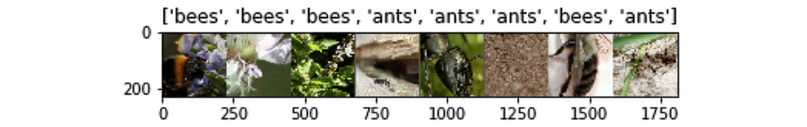
Figure 3.15 – Bees versus ants dataset
- We now define the fine-tuning routine, which is essentially a training routine performed on a pre-trained model:
def finetune_model(pretrained_model, loss_func, optim, epochs=10):
...
for e in range(epochs):
for dset in ['train', 'val']:
if dset == 'train':
pretrained_model.train() # set model to train mode (i.e. trainbale weights)
else:
pretrained_model.eval() # set model to validation mode
# iterate over the (training/validation) data.
for imgs, tgts in dloaders[dset]:
...
optim.zero_grad()
with torch.set_grad_enabled(dset == 'train'):
ops = pretrained_model(imgs)
_, preds = torch.max(ops, 1)
loss_curr = loss_func(ops, tgts)
# backward pass only if in training mode
if dset == 'train':
loss_curr.backward()
optim.step()
loss += loss_curr.item() * imgs.size(0)
successes += torch.sum(preds == tgts.data)
loss_epoch = loss / dset_sizes[dset]
accuracy_epoch = successes.double() / dset_sizes[dset]
if dset == 'val' and accuracy_epoch > accuracy:
accuracy = accuracy_epoch
model_weights = copy.deepcopy(pretrained_model.state_dict())
# load the best model version (weights)
pretrained_model.load_state_dict(model_weights)
return pretrained_model
In this function, we require the pre-trained model (that is, the architecture as well as weights) as input along with the loss function, optimizer, and number of epochs. Basically, instead of starting from a random initialization of weights, we start with the pre-trained weights of AlexNet. The other parts of this function are pretty similar to our previous exercises.
- Before starting to fine-tune (train) the model, we will define a function to visualize the model predictions:
def visualize_predictions(pretrained_model, max_num_imgs=4):
was_model_training = pretrained_model.training
pretrained_model.eval()
imgs_counter = 0
fig = plt.figure()
with torch.no_grad():
for i, (imgs, tgts) in enumerate(dloaders['val']):
imgs = imgs.to(dvc)
tgts = tgts.to(dvc)
ops = pretrained_model(imgs)
_, preds = torch.max(ops, 1)
for j in range(imgs.size()[0]):
imgs_counter += 1
ax = plt.subplot(max_num_imgs//2, 2, imgs_counter)
ax.axis('off')
ax.set_title(f'Prediction: {class_names[preds[j]]}, Ground Truth: {class_names[tgts[j]]}')
imshow(inputs.cpu().data[j])
if imgs_counter == max_num_imgs:
pretrained_model.train(mode=was_training)
return
model.train(mode=was_training)
- Finally, we get to the interesting part. Let's use PyTorch's torchvision.models sub-package to load the pre-trained AlexNet model:
model_finetune = models.alexnet(pretrained=True)
This model object has the following two main components:
i) features: The feature extraction component, which contains all the convolutional and pooling layers
ii) classifier: The classifier block, which contains all the fully connected layers leading to the output layer
- We can visualize these components as shown here:
print(model_finetune.features)
This should output the following:

Figure 3.16 – AlexNet feature extractor
- Now, we will run the classifier feature as follows:
print(model_finetune.classifier)
This should output the following:
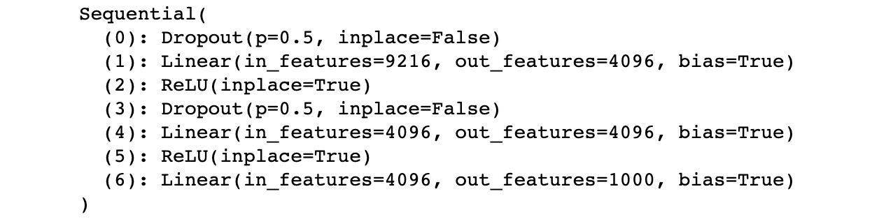
Figure 3.17 – AlexNet classifier
- As you may have noticed, the pre-trained model has the output layer of size 1000, but we only have 2 classes in our fine-tuning dataset. So, we shall alter that, as shown here:
# change the last layer from 1000 classes to 2 classes
model_finetune.classifier[6] = nn.Linear(4096, len(classes))
- And now, we are all set to define the optimizer and loss function, and thereafter run the training routine as follows:
loss_func = nn.CrossEntropyLoss()
optim_finetune = optim.SGD(model_finetune.parameters(), lr=0.0001)
# train (fine-tune) and validate the model
model_finetune = finetune_model(model_finetune, loss_func, optim_finetune, epochs=10)
The output will be as follows:

Figure 3.18 – AlexNet fine-tuning loop
- Let's visualize some of the model predictions to see whether the model has indeed learned the relevant features from this small dataset:
visualize_predictions(model_finetune)
This should output the following:

Figure 3.19 – AlexNet predictions
Clearly, the pretrained AlexNet model has been able to transfer-learn on this rather tiny image classification dataset. This both demonstrates the power of transfer learning as well as the speed and ease with which we can fine-tune well known models using PyTorch.
In the next section, we will discuss an even deeper and more complex successor of AlexNet – the VGG network. We have demonstrated the model definition, dataset loading, model training (or fine-tuning), and evaluation steps in detail for LeNet and AlexNet. In subsequent sections, we will focus mostly on model architecture definition, as the PyTorch code for other aspects (such as data loading and evaluation) will be similar.
Running a pre-trained VGG model
We have already discussed LeNet and AlexNet, two of the foundational CNN architectures. As we progress in the chapter, we will explore increasingly complex CNN models. Although, the key principles in building these model architectures will be the same. We will see a modular model-building approach in putting together convolutional layers, pooling layers, and fully connected layers into blocks/modules and then stacking these blocks sequentially or in a branched manner. In this section, we look at the successor to AlexNet – VGGNet.
The name VGG is derived from the Visual Geometry Group of Oxford University, where this model was invented. Compared to the 8 layers and 60 million parameters of AlexNet, VGG consists of 13 layers (10 convolutional layers and 3 fully connected layers) and 138 million parameters. VGG basically stacks more layers onto the AlexNet architecture with smaller size convolution kernels (2x2 or 3x3). Hence, VGG's novelty lies in the unprecedented level of depth that it brings with its architecture. Figure 3.20 shows the VGG architecture:

Figure 3.20 – VGG16 architecture
The preceding VGG architecture is called VGG13, because of the 13 layers. Other variants are VGG16 and VGG19, consisting of 16 and 19 layers, respectively. There is another set of variants – VGG13_bn, VGG16_bn, and VGG19_bn, where bn suggests that these models also consist of batch-normalization layers.
PyTorch's torchvision.model sub-package provides the pre-trained VGG model (with all of the six variants discussed earlier) trained on the ImageNet dataset. In the following exercise, we will use the pre-trained VGG13 model to make predictions on a small dataset of bees and ants (used in the previous exercise). We will focus on the key pieces of code here, as most other parts of our code will overlap with that of the previous exercises. We can always refer to our notebooks to explore the full code: https://github.com/PacktPublishing/Mastering-PyTorch/blob/master/Chapter03/vgg13_pretrained_run_inference.ipynb:
- First, we need to import dependencies, including torchvision.models.
- Download the data and set up the ants and bees dataset and dataloader, along with the transformations.
- In order to make predictions on these images, we will need the 1,000 labels of the ImageNet dataset, which can be found here: https://gist.github.com/yrevar/942d3a0ac09ec9e5eb3a.
- Once downloaded, we need to create a mapping between the class indices 0 to 999 and the corresponding class labels, as shown here:
import ast
with open('./imagenet1000_clsidx_to_labels.txt') as f:
classes_data = f.read()
classes_dict = ast.literal_eval(classes_data)
print({k: classes_dict[k] for k in list(classes_dict)[:5]})
This should output the first five class mappings, as shown in the following screenshot:

Figure 3.21 – ImageNet class mappings
- Define the model prediction visualization function that takes in the pre-trained model object and the number of images to run predictions on. This function should output the images with predictions.
- Load the pretrained VGG13 model:
model_finetune = models.vgg13(pretrained=True)
This should output the following:

Figure 3.22 – Loading the VGG13 model
The 508 MB VGG13 model is downloaded in this step.
- Finally, we run predictions on our ants and bees dataset using this pre-trained model:
visualize_predictions(model_finetune)
This should output the following:

Figure 3.23 – VGG13 predictions
The VGG13 model trained on an entirely different dataset seems to predict all the test samples correctly in the ants and bees dataset. Basically, the model grabs the two most similar animals from the dataset out of the 1,000 classes and finds them in the images. By doing this exercise, we see that the model is still able to extract relevant visual features out of the images and the exercise demonstrates the utility of PyTorch's out-of-the-box inference feature.
In the next section, we are going to study a different type of CNN architecture – one that involves modules that have multiple parallel convolutional layers. The modules are called Inception modules and the resulting network is called the Inception network. We will explore the various parts of this network and the reasoning behind its success. We will also build the inception modules and the Inception network architecture using PyTorch.
Exploring GoogLeNet and Inception v3
As we have discovered the progression of CNN models from LeNet to VGG so far, we have observed the sequential stacking of more convolutional and fully connected layers. This resulted in deep networks with a lot of parameters to train. GoogLeNet emerged as a radically different type of CNN architecture that is composed of a module of parallel convolutional layers called the inception module. Because of this, GoogLeNet is also called Inception v1 (v1 marked the first version as more versions came along later). Some of the drastically new elements introduced in GoogLeNet were the following:
- The inception module – a module of several parallel convolutional layers
- Using 1x1 convolutions to reduce the number of model parameters
- Global average pooling instead of a fully connected layer – reduces overfitting
- Using auxiliary classifiers for training – for regularization and gradient stability
GoogLeNet has 22 layers, which is more than the number of layers of any VGG model variant. Yet, due to some of the optimization tricks used, the number of parameters in GoogLeNet is 5 million, which is far less than the 138 million parameters of VGG. Let's expand on some of the key features of this model.
Inception modules
Perhaps the single most important contribution of this model was the development of a convolutional module with several convolutional layers running in parallel, which are finally concatenated to produce a single output vector. These parallel convolutional layers operate with different kernel sizes ranging from 1x1 to 3x3 to 5x5. The idea is to extract all levels of visual information from the image. Besides these convolutions, a 3x3 max-pooling layer adds another level of feature extraction. Figure 3.24 shows the inception block diagram along with the overall GoogLeNet architecture:

Figure 3.24 – GoogLeNet architecture
By using this architecture diagram, we can build the inception module in PyTorch as shown here:
class InceptionModule(nn.Module):
def __init__(self, input_planes, n_channels1x1, n_channels3x3red, n_channels3x3, n_channels5x5red, n_channels5x5, pooling_planes):
super(InceptionModule, self).__init__()
# 1x1 convolution branch
self.block1 = nn.Sequential(
nn.Conv2d(input_planes, n_channels1x1, kernel_size=1),nn.BatchNorm2d(n_channels1x1),nn.ReLU(True),)
# 1x1 convolution -> 3x3 convolution branch
self.block2 = nn.Sequential(
nn.Conv2d(input_planes, n_channels3x3red, kernel_size=1),nn.BatchNorm2d(n_channels3x3red),
nn.ReLU(True),nn.Conv2d(n_channels3x3red, n_channels3x3, kernel_size=3, padding=1),nn.BatchNorm2d(n_channels3x3),nn.ReLU(True),)
# 1x1 conv -> 5x5 conv branch
self.block3 = nn.Sequential(
nn.Conv2d(input_planes, n_channels5x5red, kernel_size=1),nn.BatchNorm2d(n_channels5x5red),nn.ReLU(True),
nn.Conv2d(n_channels5x5red, n_channels5x5, kernel_size=3, padding=1),nn.BatchNorm2d(n_channels5x5),nn.ReLU(True),
nn.Conv2d(n_channels5x5, n_channels5x5, kernel_size=3, padding=1),nn.BatchNorm2d(n_channels5x5),
nn.ReLU(True),)
# 3x3 pool -> 1x1 conv branch
self.block4 = nn.Sequential(
nn.MaxPool2d(3, stride=1, padding=1),
nn.Conv2d(input_planes, pooling_planes, kernel_size=1),
nn.BatchNorm2d(pooling_planes),
nn.ReLU(True),)
def forward(self, ip):
op1 = self.block1(ip)
op2 = self.block2(ip)
op3 = self.block3(ip)
op4 = self.block4(ip)
return torch.cat([op1,op2,op3,op4], 1)
Next, we will look at another important feature of GoogLeNet – 1x1 convolutions.
1x1 convolutions
In addition to the parallel convolutional layers in an inception module, each parallel layer has a preceding 1x1 convolutional layer. The reason behind using these 1x1 convolutional layers is dimensionality reduction. 1x1 convolutions do not change the width and height of the image representation but can alter the depth of an image representation. This trick is used to reduce the depth of the input visual features before performing the 1x1, 3x3, and 5x5 convolutions parallelly. Reducing the number of parameters not only helps build a lighter model but also combats overfitting.
Global average pooling
If we look at the overall GoogLeNet architecture in Figure 3.24, the penultimate output layer of the model is preceded by a 7x7 average pooling layer. This layer again helps in reducing the number of parameters of the model, thereby reducing overfitting. Without this layer, the model would have millions of additional parameters due to the dense connections of a fully connected layer.
Auxiliary classifiers
Figure 3.24 also shows two extra or auxiliary output branches in the model. These auxiliary classifiers are supposed to tackle the vanishing gradient problem by adding to the gradients' magnitude during backpropagation, especially for the layers towards the input end. Because these models have a large number of layers, vanishing gradients can become a bottleneck. Hence, using auxiliary classifiers has proven useful for this 22-layer deep model. Additionally, the auxiliary branches also help in regularization. Please note that these auxiliary branches are switched off/discarded while making predictions.
Once we have the inception module defined using PyTorch, we can easily instantiate the entire Inception v1 model as follows:
class GoogLeNet(nn.Module):
def __init__(self):
super(GoogLeNet, self).__init__()
self.stem = nn.Sequential(
nn.Conv2d(3, 192, kernel_size=3, padding=1),
nn.BatchNorm2d(192),
nn.ReLU(True),)
self.im1 = InceptionModule(192, 64, 96, 128, 16, 32, 32)
self.im2 = InceptionModule(256, 128, 128, 192, 32, 96, 64)
self.max_pool = nn.MaxPool2d(3, stride=2, padding=1)
self.im3 = InceptionModule(480, 192, 96, 208, 16, 48, 64)
self.im4 = InceptionModule(512, 160, 112, 224, 24, 64, 64)
self.im5 = InceptionModule(512, 128, 128, 256, 24, 64, 64)
self.im6 = InceptionModule(512, 112, 144, 288, 32, 64, 64)
self.im7 = InceptionModule(528, 256, 160, 320, 32, 128, 128)
self.im8 = InceptionModule(832, 256, 160, 320, 32, 128, 128)
self.im9 = InceptionModule(832, 384, 192, 384, 48, 128, 128)
self.average_pool = nn.AvgPool2d(7, stride=1)
self.fc = nn.Linear(4096, 1000)
def forward(self, ip):
op = self.stem(ip)
out = self.im1(op)
out = self.im2(op)
op = self.maxpool(op)
op = self.a4(op)
op = self.b4(op)
op = self.c4(op)
op = self.d4(op)
op = self.e4(op)
op = self.max_pool(op)
op = self.a5(op)
op = self.b5(op)
op = self.avgerage_pool(op)
op = op.view(op.size(0), -1)
op = self.fc(op)
return op
Besides instantiating our own model, we can always load a pre-trained GoogLeNet with just two lines of code:
import torchvision.models as models
model = models.googlenet(pretrained=True)
Finally, as mentioned earlier, a number of versions of the Inception model were developed later. One of the eminent ones was Inception v3, which we will briefly discuss next.
Inception v3
This successor of Inception v1 has a total of 24 million parameters as compared to 5 million in v1. Besides the addition of several more layers, this model introduced different kinds of inception modules, which are stacked sequentially. Figure 3.25 shows the different inception modules and the full model architecture:

Fig 3.25 – Inception v3 architecture
It can be seen from the architecture that this model is an architectural extension of the Inception v1 model. Once again, besides building the model manually, we can use the pre-trained model from PyTorch's repository as follows:
import torchvision.models as models
model = models.inception_v3(pretrained=True)
In the next section, we will go through the classes of CNN models that have effectively combatted the vanishing gradient problem in very deep CNNs – ResNet and DenseNet. We will learn about the novel techniques of skip connections and dense connections and use PyTorch to code the fundamental modules behind these advanced architectures.
Discussing ResNet and DenseNet architectures
In the previous section, we explored the Inception models, which had a reduced number of model parameters as the number of layers increased, thanks to the 1x1 convolutions and global average pooling. Furthermore, auxiliary classifiers were used to combat the vanishing gradient problem.
ResNet introduced the concept of skip connections. This simple yet effective trick overcomes the problem of both parameter overflow and vanishing gradients. The idea, as shown in the following diagram, is quite simple. The input is first passed through a non-linear transformation (convolutions followed by non-linear activations) and then the output of this transformation (referred to as the residual) is added to the original input. Each block of such computation is called a residual block, hence the name of the model – residual network or ResNet.

Figure 3.26 – Skip connections
Using these skip (or shortcut) connections, the number of parameters is limited to 26 million parameters for a total of 50 layers (ResNet-50). Due to the limited number of parameters, ResNet has been able to generalize well without overfitting even when the number of layers is increased to 152 (ResNet-152). The following diagram shows the ResNet-50 architecture:

Figure 3.27 – ResNet architecture
There are two kinds of residual blocks – convolutional and identity, both having skip connections. For the convolutional block, there is an added 1x1 convolutional layer, which further helps to reduce dimensionality. A residual block for ResNet can be implemented in PyTorch as shown here:
class BasicBlock(nn.Module):
multiplier=1
def __init__(self, input_num_planes, num_planes, strd=1):
super(BasicBlock, self).__init__()
self.conv_layer1 = nn.Conv2d(in_channels=input_num_planes, out_channels=num_planes, kernel_size=3, stride=stride, padding=1, bias=False)
self.batch_norm1 = nn.BatchNorm2d(num_planes)
self.conv_layer2 = nn.Conv2d(in_channels=num_planes, out_channels=num_planes, kernel_size=3, stride=1, padding=1, bias=False)
self.batch_norm2 = nn.BatchNorm2d(num_planes)
self.res_connnection = nn.Sequential()
if strd > 1 or input_num_planes != self.multiplier*num_planes:
self.res_connnection = nn.Sequential(
nn.Conv2d(in_channels=input_num_planes, out_channels=self.multiplier*num_planes, kernel_size=1, stride=strd, bias=False),
nn.BatchNorm2d(self.multiplier*num_planes))
def forward(self, inp):
op = F.relu(self.batch_norm1(self.conv_layer1(inp)))
op = self.batch_norm2(self.conv_layer2(op))
op += self.res_connnection(inp)
op = F.relu(op)
return op
To get started quickly with ResNet, we can always use the pre-trained ResNet model from PyTorch's repository:
import torchvision.models as models
model = models.resnet50(pretrained=True)
ResNet uses the identity function (by directly connecting input to output) to preserve the gradient during backpropagation (as the gradient will be 1). Yet, for extremely deep networks, this principle might not be sufficient to preserve strong gradients from the output layer back to the input layer.
The CNN model we will discuss next is designed to ensure a strong gradient flow, as well as a further reduction in the number of required parameters.
DenseNet
The skip connections of ResNet connected the input of a residual block directly to its output. However, the inter-residual-blocks connection is still sequential, that is, residual block number 3 has a direct connection with block 2 but no direct connection with block 1.
DenseNet, or dense networks, introduced the idea of connecting every convolutional layer with every other layer within what is called a dense block. And every dense block is connected to every other dense block in the overall DenseNet. A dense block is simply a module of two 3x3 densely connected convolutional layers.
These dense connections ensure that every layer is receiving information from all of the preceding layers of the network. This ensures that there is a strong gradient flow from the last layer down to the very first layer. Counterintuitively, the number of parameters of such a network setting will also be low. As every layer is receiving the feature maps from all the previous layers, the required number of channels (depth) can be fewer. In the earlier models, the increasing depth represented the accumulation of information from earlier layers, but we don't need that anymore, thanks to the dense connections everywhere in the network.
One key difference between ResNet and DenseNet is also that, in ResNet, the input was added to the output using skip connections. But in the case of DenseNet, the preceding layers' outputs are concatenated with the current layer's output. And the concatenation happens in the depth dimension.
This might raise a question about the exploding size of outputs as we proceed further in the network. To combat this compounding effect, a special type of block called the transition block is devised for this network. Composed of a 1x1 convolutional layer followed by a 2x2 pooling layer, this block standardizes or resets the size of the depth dimension so that the output of this block can then be fed to the subsequent dense block(s). The following diagram shows the DenseNet architecture:

Figure 3.28 – DenseNet architecture
As mentioned earlier, there are two types of blocks involved – the dense block and the transition block. These blocks can be written as classes in PyTorch in a few lines of code, as shown here:
class DenseBlock(nn.Module):
def __init__(self, input_num_planes, rate_inc):
super(DenseBlock, self).__init__()
self.batch_norm1 = nn.BatchNorm2d(input_num_planes)
self.conv_layer1 = nn.Conv2d(in_channels=input_num_planes, out_channels=4*rate_inc, kernel_size=1, bias=False)
self.batch_norm2 = nn.BatchNorm2d(4*rate_inc)
self.conv_layer2 = nn.Conv2d(in_channels=4*rate_inc, out_channels=rate_inc, kernel_size=3, padding=1, bias=False)
def forward(self, inp):
op = self.conv_layer1(F.relu(self.batch_norm1(inp)))
op = self.conv_layer2(F.relu(self.batch_norm2(op)))
op = torch.cat([op,inp], 1)
return op
class TransBlock(nn.Module):
def __init__(self, input_num_planes, output_num_planes):
super(TransBlock, self).__init__()
self.batch_norm = nn.BatchNorm2d(input_num_planes)
self.conv_layer = nn.Conv2d(in_channels=input_num_planes, out_channels=output_num_planes, kernel_size=1, bias=False)
def forward(self, inp):
op = self.conv_layer(F.relu(self.batch_norm(inp)))
op = F.avg_pool2d(op, 2)
return op
These blocks are then stacked densely to form the overall DenseNet architecture. DenseNet, like ResNet, comes in variants such as DenseNet121, DenseNet161, DenseNet169, and DenseNet201, where the numbers represent the total number of layers. Such large numbers of layers are obtained by the repeated stacking of the dense and transition blocks plus a fixed 7x7 convolutional layer at the input end and a fixed fully connected layer at the output end. PyTorch provides pre-trained models for all of these variants:
import torchvision.models as models
densenet121 = models.densenet121(pretrained=True)
densenet161 = models.densenet161(pretrained=True)
densenet169 = models.densenet169(pretrained=True)
densenet201 = models.densenet201(pretrained=True)
DenseNet outperforms all the models discussed so far on the ImageNet dataset. Various hybrid models have been developed by mixing and matching the ideas presented in the previous sections. The Inception-ResNet and ResNeXt models are examples of such hybrid networks. The following diagram shows the ResNeXt architecture:
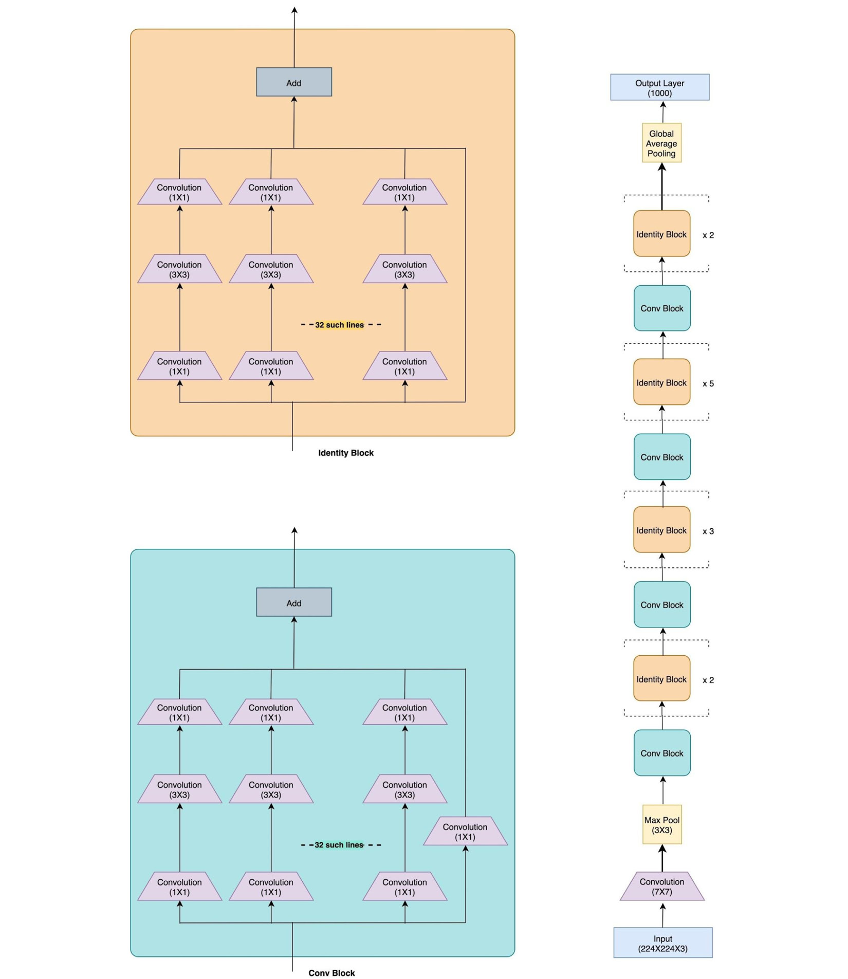
Figure 3.29 – ResNeXt architecture
As you can see, it looks like a wider variant of a ResNet + Inception hybrid because there is a large number of parallel convolutional branches in the residual blocks – and the idea of parallelism is derived from the inception network.
In the next and last section of this chapter, we are going to look at the current best performing CNN architectures – EfficientNets. We will also discuss the future of CNN architectural development while touching upon the use of CNN architectures for tasks beyond image classification.
Understanding EfficientNets and the future of CNN architectures
So far in our exploration from LeNet to DenseNet, we have noticed an underlying theme in the advancement of CNN architectures. That theme is the expansion or scaling of the CNN model through one of the following:
- An increase in the number of layers
- An increase in the number of feature maps or channels in a convolutional layer
- An increase in the spatial dimension going from 32x32 pixel images in LeNet to 224x224 pixel images in AlexNet and so on
These three different aspects on which scaling can be performed are identified as depth, width, and resolution, respectively. Instead of manually scaling these attributes, which often leads to suboptimal results, EfficientNets use neural architecture search to calculate the optimal scaling factors for each of them.
Scaling up depth is deemed important because the deeper the network, the more complex the model, and hence it can learn highly complex features. However, there is a trade-off because, with increasing depth, the vanishing gradient problem escalates along with the general problem of overfitting.
Similarly, scaling up width should theoretically help, as with a greater number of channels, the network should learn more fine-grained features. However, for extremely wide models, the accuracy tends to saturate quickly.
Finally, higher resolution images, in theory, should work better as they have more fine-grained information. Empirically, however, the increase in resolution does not yield a linearly equivalent increase in the model performance. All of this is to say that there are trade-offs to be made while deciding the scaling factors and hence, neural architecture search helps in finding the optimal scaling factors.
EfficientNet proposes finding the architecture that has the right balance between depth, width, and resolution, and all three of these aspects are scaled together using a global scaling factor. The EfficientNet architecture is built in two steps. First, a basic architecture (called the base network) is devised by fixing the scaling factor to 1. At this stage, the relative importance of depth, width, and resolution is decided for the given task and dataset. The base network obtained is pretty similar to a well-known CNN architecture – MnasNet, short for Mobile Neural Architecture Search Network. PyTorch offers the pre-trained MnasNet model, which can be loaded as shown here:
import torchvision.models as models
model = models.mnasnet1_0()
Once the base network is obtained in the first step, the optimal global scaling factor is then computed with the aim of maximizing the accuracy of the model and minimizing the number of computations (or flops). The base network is called EfficientNet B0 and the subsequent networks derived for different optimal scaling factors are called EfficientNet B1-B7.
As we go forward, efficient scaling of CNN architecture is going to be a prominent direction of research along with the development of more sophisticated modules inspired by the inception, residual, and dense modules. Another aspect of CNN architecture development is minimizing the model size while retaining performance. MobileNets (https://pytorch.org/hub/pytorch_vision_mobilenet_v2/) are a prime example and there is a lot of ongoing research on this front.
Besides the top-down approach of looking at architectural modifications of a pre-existing model, there will be continued efforts adopting the bottom-up view of fundamentally rethinking the units of CNNs such as the convolutional kernels, pooling mechanism, more effective ways of flattening, and so on. One concrete example of this could be CapsuleNet (https://en.wikipedia.org/wiki/Capsule_neural_network), which revamped the convolutional units to cater to the third dimension (depth) in images.
CNNs are a huge topic of study in themselves. In this chapter, we have touched upon the architectural development of CNNs, mostly in the context of image classification. However, these same architectures are used across a wide variety of applications. One well-known example is the use of ResNets for object detection and segmentation in the form of RCNNs (https://en.wikipedia.org/wiki/Region_Based_Convolutional_Neural_Networks). Some of the improved variants of RCNNs are Faster R-CNN, Mask-RCNN, and Keypoint-RCNN. PyTorch provides pre-trained models for all three variants:
faster_rcnn = models.detection.fasterrcnn_resnet50_fpn()
mask_rcnn = models.detection.maskrcnn_resnet50_fpn()
keypoint_rcnn = models.detection.keypointrcnn_resnet50_fpn()
PyTorch also provides pre-trained models for ResNets that are applied to video-related tasks such as video classification. Two such ResNet-based models used for video classification are ResNet3D and ResNet Mixed Convolution:
resnet_3d = models.video.r3d_18()
resnet_mixed_conv = models.video.mc3_18()
While we do not extensively cover these different applications and corresponding CNN models in this chapter, we encourage you to read more on them. PyTorch's website can be a good starting point: https://pytorch.org/docs/stable/torchvision/models.html#object-detection-instance-segmentation-and-person-keypoint-detection.
Summary
This chapter has been all about CNN architectures. First, we briefly discussed the history and evolution of CNNs. We then explored in detail one of the earliest CNN models – LeNet. Using PyTorch, we built the model from scratch and trained and tested it on an image classification dataset. We then explored LeNet's successor – AlexNet. Instead of building it from scratch, we used PyTorch's pre-trained model repository to load a pre-trained AlexNet model. We then fine-tuned the loaded model on a different dataset and evaluated its performance.
Next, we looked at the VGG model, which is a deeper and a more advanced successor to AlexNet. We loaded a pre-trained VGG model using PyTorch and used it to make predictions on a different image classification dataset. We then successively discussed the GoogLeNet and Inception v3 models that are composed of several inception modules. Using PyTorch, we wrote the implementation of an inception module and the whole network. Moving on, we discussed ResNet and DenseNet. For each of these architectures, we implemented their building blocks, that is, residual blocks and dense blocks, using PyTorch. We also briefly looked at an advanced hybrid CNN architecture – ResNeXt.
Finally, we concluded the chapter with an overview of the current state-of-the-art CNN model – EfficientNet. We discussed the idea behind it and the related pre-trained models available under PyTorch, such as MnasNet. We also provided plausible future directions for CNN architectural developments, along with briefly mentioning other CNN architectures specific to object detection and video classification, such as RCNNs and ResNet3D respectively.
Although this chapter does not cover every possible topic under the concept of CNN architectures, it still provides an elaborate understanding of the progression of CNNs from LeNet to EfficientNet and beyond. Moreover, this chapter highlights the effective use and application of PyTorch for the various CNN architectures that we have discussed.
In the next chapter, we will explore a similar journey but for another important type of neural network – recurrent neural networks. We will discuss the various recurrent net architectures and use PyTorch to effectively implement, train, and test them.