Chapter 3: DS2 Data Program Details

3.1 Introduction

3.2 DS2 Data Programs versus Base SAS DATA Steps

3.2.1 General Considerations

3.2.2 The Seven Subtle Dissimilarities

3.2.3 DS2 “Missing” Features

3.3 Data Types in DS2

3.3.1 DS2 and ANSI Data Types

3.3.2 Automatic Data Type Conversion

3.3.3 Non-coercible Data Types

3.3.4 Processing SAS Missing and ANSI Null Values

3.4 Review of Key Concepts

3.1 Introduction

In this chapter, we’ll focus on DS2 data program fundamentals, first by further comparing and contrasting the traditional DATA step with the DS2 data program, and then by diving into some of the things that are new in DS2. In the process, we’ll convert more complex Base SAS DATA steps into DS2 data programs, and we will introduce several concepts and techniques that are unique to DS2. Specifically, we will cover these points:

●   more DS2 data program syntax and structure

●   using FedSQL queries to provide input directly to a DS2 data program SET statement

●   the wide variety of ANSI data types that can be processed in DS2

●   DS2 automatic data type conversion rules

●   unique DS2 program statements

●   unique DS2 expressions

●   selected DS2 functions

3.2 DS2 Data Programs versus Base SAS DATA Steps

3.2.1 General Considerations

The DS2 data program syntax’s similarity to Base SAS DATA step syntax is an advantage for seasoned SAS programmers. This similarity clearly shows in the statement syntax that is shared between the Base SAS DATA step and the DS2 data program. For example, these statements work essentially the same in both languages:

●   SET

●   BY-group processing, including First.variable and Last.variable

●   DO groups and DO loops

◦   DO i= start TO stop BY interval

◦   DO WHILE ()

◦   DO UNTIL ()

◦   loop flow control statements CONTINUE, LEAVE, and END

●   Program flow control statements

◦   RETURN

◦   OUTPUT

◦   GOTO

◦   STOP

●   Declarative statements

◦   KEEP and DROP

◦   RETAIN

Remember that in any DS2 program, global declarative statements must appear in the global program space—that is, after the DATA, THREAD, or PACKAGE statement and before the first method definition.

In addition to supporting many traditional DATA step statements, DS2 also supports most traditional DATA step variable lists, such as numbered range and prefix lists, as well as lists based on data type. Variable lists can save us a lot of typing (and typos!) when writing DS2 programs, so it’s worth our time to do a quick review here. While we’re at it, we’ll highlight a small difference in DS2 and traditional DATA step data type-based lists. For the purposes of our discussion of variable lists, we will assume that the DS2 data program in which the list is used starts with a PDV that looks like this:

A name variable list is just a list of existing global variable names, for example:

The output data set would have this structure:

A numbered range variable list references global variables with a specific prefix and a numeric suffix between the specified numbers, for example:

When these lists are expanded by the compiler, variable names are constructed by concatenating the prefix with each number in the numbered range. For example, the above numbered range lists, when expanded, are equivalent to:

The output data set would have this structure:

A name range variable list references all global variables whose position in the PDV falls between the two specified variables, inclusive, for example:

The above name range list, when expanded, is equivalent to:

The output data set would have this structure:

A name prefix variable references all global variables that begin with a specified prefix, for example:

The above name prefix list, when expanded, is equivalent to:

The output data set would have this structure:

A type variable references all global variables of a specified type. In the traditional DATA step, there are two special variable lists based on data type: _numeric_ and _character_. Because DS2 has a much richer data type palette, those old lists don’t work in DS2. Instead, just use the data type name as the list. For example:

The above list, when expanded, is equivalent to:

The output data set would have this structure:

With SAS 9.4M5, variable lists are much more useful, because most functions now support the OF operator. For example:

As a bonus, you can also use an array reference as a variable list, for example:

3.2.2 The Seven Subtle Dissimilarities

Though many things work exactly the same in a traditional DATA step and a DS2 data program, some differences can be quite subtle and must be kept in mind by DS2 programmers. Let’s go over the primary culprits, which I’ve come to refer to as the seven subtle dissimilarities.

3.2.2.1 Dissimilarity 1: All Executable Statements Must Be Part of a Method Code Block

Executable statements in the global program space result in a syntax error:

SAS Log:

Enclosing the executable statements in a method resolves the issue:

SAS Log:

3.2.2.2 Dissimilarity 2: DS2 Programs Do Not Overwrite Data by Default

If you submit this program once, it runs normally. If you submit the exact same program a second time, it results in a syntax error:

SAS Log:

You can control this behavior using the OVERWRITE=YES option in the DATA statement, or the OVERWRITE=YES table option. The table option enables overwriting only the data set specifying the option. The DATA statement option enables overwriting of all the output tables listed in the DATA statement. For example, this program resolves the issue with data set test1, but because data set test2 is not allowed to be overwritten, we still get a compilation error:

SAS Log:

Using the DATA statement OVERWRITE=YES option enables overwriting of both tables:

SAS Log:

As a matter of fact, in keeping with its tighter integration with ANSI systems, you can’t read from and write to a data set simultaneously with a DS2 DATA program as you can with a traditional DATA step:

SAS Log:

3.2.2.3 Dissimilarity 3: All Variables Not Introduced via the SET Statement Should Be Declared

By default, failure to declare a new variable results in a warning in the SAS log. This behavior can be controlled globally with the SAS system option DS2SCOND. The system option can be overridden for a particular DS2 instance using the PROC DS2 option SCOND or a DS2_OPTIONS statement.

Table 3.1: DS2SCOND and SCOND Option Values and Effects

Option Setting	Effect for Undeclared Variables
NONE	Program compiles and executes normally. There is no entry in the log.
NOTE	Program compiles and executes normally. A note is generated in the SAS log for each undeclared variable.
WARNING(default)	Program compiles and executes normally. A warning is generated in the SAS log for each undeclared variable.
ERROR	An error is generated in the SAS log for each undeclared variable. Program fails to compile and will not execute.

Here is an example of setting the system option DS2SCOND to ERROR:

SAS Log:

Here is an example of overriding the system option setting using the PROC DS2 option SCOND:

SAS Log:

And finally, here is an example of overriding the system option setting using a DS2_OPTIONS statement:

SAS Log:

3.2.2.4 Dissimilarity 4: PUT Statement Cursor and Line Pointers Are Not Supported

The following Base SAS DATA step writes neatly organized information in the log using cursor controls (@) and line feeds (/):

SAS Log:

However, the same code in DS2 generates syntax errors, because the PUT statement in DS2 does not accept cursor and line controls:

SAS Log:

3.2.2.5 Dissimilarity 5: Keywords Are Reserved Words

The Base SAS DATA step language has very few reserved words. By examining the context, the compiler decides whether a keyword should be interpreted as code or as an identifier. For example, it is perfectly OK to name your data set Data or a variable Character:

SAS Log:

However, the same code in DS2 generates syntax errors, because in DS2 all keywords are reserved:

Following ANSI SQL standards, you can use a keyword as an identifier only if you enclose it in double quotation marks:

SAS Log:

3.2.2.6 Dissimilarity 6: DS2 Uses ANSI SQL Quoting Standards

In DS2, double quotation marks are used only to delimit an identifier. Single quotation marks are required to delimit constants:

SAS Log:

This requirement can be problematic when trying to resolve macro variables as all or part of a character constant value in DS2. If the macro reference is placed in the single quotation marks that are required for constant text in DS2, the macro variable fails to resolve. That is because single quotation marks prevent tokenization of the enclosed text:

SAS Log:

If you place the macro reference in double quotation marks so that it can be tokenized and resolved, DS2 interprets the resolved text as an identifier instead of constant text:

SAS Log:

As we can see from the log, DS2 interpreted “This is the message.” as a variable name. Because there was no indication of what type of variable to create, DS2 created a double-precision, floating-point numeric (SAS numeric) variable name “this is the message.” The value of this new variable was assigned to the “Character” variable, which is a text variable. The automatic conversion from numeric missing to character produced the ‘.’ that we then see printed in the log. We can tell what happened because of the warning message produced by the use of an undeclared variable.

To facilitate including macro-generated text in DS2 literals, SAS provides the autocall macro %TSLIT. %TSLIT first enables all macro triggers to resolve, and then takes the resulting text and applies a real single quotation mark character to the beginning and to the end of the text string. Finally, SAS sends the resulting text back to the word scanner. This makes macro variable resolution work as expected in DS2:

SAS Log:

3.2.2.7 Dissimilarity 7: MERGE Statement Disparities

The Base SAS DATA step MERGE processing fundamentally differs from the SQL join. The DS2 MERGE statement differs from both. Before using MERGE in DS2, it is important to understand the behavior and expected output. Let’s look at the output from all three methods when assembling data from two tables with one-to-one, one-to-many, and many-to-many relationships between rows.

These are the source data sets used in the following examples:

Figure 3.1: Source Data Sets Used for Join vs. Merge Comparisons

Because the SQL full join produces output most closely resembling the default output from a traditional DATA step merge, we’ll compare the result of a traditional DATA step merge vs. a DS2 merge vs. an SQL full join. Later in this book, we will investigate how DS2 integrates with SQL. However, the SQL used in conjunction with DS2 is not the venerable PROC SQL, but a newer version of SQL based on the more modern ANSI 1999 standard called Federated SQL (FedSQL). You can write stand-alone queries using the new SQL by invoking PROC FedSQL instead of PROC SQL. There is excellent and extensive documentation available for FedSQL in SAS 9.4 FedSQL Language Reference. The following examples all use PROC FedSQL, but the queries shown will produce identical results when executed using PROC SQL.

3.2.2.7.1 Simple MERGE Scenarios

Using the data sets described in the previous paragraph, let’s first conduct our experiment on tables A and B, which have a simple, one-to-one relationship.

Figure 3.2: One-to-One: DATA step Merge vs. DS2 Merge vs. SQL Join  

As you can see, in a one-to-one situation all processes produce identical results. Next, let’s experiment on tables A and C, with their one-to-many relationship.

Figure 3.3: One-to-Many: DATA step Merge vs. DS2 Merge vs. SQL Join

In this scenario, the traditional merge and the SQL join produced identical results, but the DS2 merge did not. Notice how the value of AVal was not retained in the PDV until the BY group changed, as it is in the traditional DATA step. Nor were the results sourced from a theoretical cartesian join of the tables, as they were in SQL.  

Finally, let’s conduct our experiment on tables C and D, which have a many-to-many relationship.

Figure 3.4: Many-to-Many: DATA step Merge vs. DS2 Merge vs. SQL Join

In this scenario, none of the processes produces identical results. The DS2 merge does not retain the value CVal until BY-group processing is complete, nor does it adopt SQL’s process of selecting rows from the Cartesian product which would have produced additional rows of output.  

3.2.2.7.2 Sparse MERGE Scenarios

Let’s move on now to highlighting the differences between the traditional DATA step MERGE and the DS2 data program MERGE. First, we’ll modify the input data sets a bit to provide a better look at sparse merges, where some rows of each table do not match any row in the other.

Figure 3.5: Source Data Sets Used for Sparse Join vs. Merge Comparisons

Using these new data sets, let’s revisit our first experiment on tables A and B, which now have a sparse one-to-one relationship. We’ll add a couple of new variables to the output to allow us to monitor the behavior of the IN= variables during the merge.

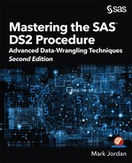
Figure 3.6: Sparse One-to-One: DATA step Merge vs. DS2 Merge

Once again, in a one-to-one situation, these processes produce identical results, and the IN= variables appear to be functioning as expected.

Next, let’s conduct the experiment on tables A and C with a one-to-many relationship.

Figure 3.7: Sparse One-to-Many: DATA step Merge vs. DS2 Merge

As expected, the traditional DATA step and DS2 merges do not produce the same results due to the lack of PDV retention for rows from table A until BY-group processing is complete. You can see that this DS2 “attitude” is also reflected in the values for the IN= variables. In a traditional DATA step merge, a single row in one table provides values to multiple output rows. As long as the BY variable values continue to match those in the incoming rows of the other table, the IN= variable value remains 1 and the PDV variable values are not reinitialized. In DS2 this is no longer true. Even though the BY group has not yet changed, because no additional rows are available in table A, the IN= variable value was set to 0 and the PDV was purged of values provided by table A.

Finally, let’s conduct our experiment on tables C and D with a sparse, many-to-many relationship.

Figure 3.8: Sparse Many-to-Many: DATA step Merge vs. DS2 Merge vs. SQL Join

In this scenario, the disparity between the traditional DATA step merge and the DS2 merge is even more prominent. Row order within BY groups is not guaranteed by DS2, even when the data sets are physically sorted in the desired order. In Figure 3.8 above, the rows associated with ID #2 tell the story. The traditional DATA step merge matched the first row in table C with an ID value of 2 to the first row in table D with an ID value of 2. This was not true for the DS2 merge. The DS2 merge matched the first row in table C with an ID value of 2 to the second row in table D with an ID value of 2. The BY-group values do match, but the order of the rows that were merged within the BY group is not what you would have expected as a traditional DATA step programmer.

3.2.3 DS2 “Missing” Features

Although the similarity of DS2 data program syntax to that of the Base SAS DATA step is helpful in getting us started with DS2 programming, eventually you will notice that several of your beloved DATA step statements and functions are not available in DS2. You’ll also notice that several new, unfamiliar statements and functions will pop up in the DS2 lexicon. In most cases, there is no loss of functionality–DS2 merely has a different approach to resolving the problem. We will examine several cases where it appears that Base SAS DATA step functionality has been lost, as well as the new approaches that DS2 takes to get the job done.

3.2.3.1 WHERE Statement

I was shocked when I realized that DS2 did not include a WHERE statement.

SAS Log:

I couldn’t find a WHERE statement in any of the DS2 documentation. But while researching this “problem” I made a delightful discovery—DS2 allows you to write an SQL query right in the SET statement, ingesting the SQL result set just as if it were a data set! Now I began to understand just what “tight integration between DS2 and SQL” could accomplish. For example, I can join data sets, then use a SET statement to ingest the SQL result set and perform DATA-step style BY-group processing. In DS2, the data program BY statement not only creates the first. and last. variables, it also enforces input data order, so there is no need to presort the input data. Using this technique, I can produce detail and summary output data sets, all in a single DS2 data program step:

SAS Log:

Figure 3.9: Detail Data Set Produced by the DS2 Data Program

Figure 3.10: Summary Data Set Produced by the DS2 Data Program

This is a significant improvement over the traditional DATA step language! It opens up some amazing opportunities to write more compact and efficient programs. Remember that the SQL used in conjunction with DS2 is FedSQL, which differs from PROC SQL, the traditional stand-alone version of SQL used in past versions of SAS. I highly recommend reading through the SAS 9.4 FedSQL Language Reference to familiarize yourself with this version of SQL.

3.2.3.2 UPDATE and MODIFY Statements

DS2 includes neither an UPDATE nor a MODIFY statement. You can produce the same effects with a little additional coding using the SQLSTMT package. We’ll show you more about that when we discuss predefined packages in Chapter 5.

3.2.3.3 ATTRIB, LABEL, LENGTH, FORMAT, and INFORMAT Statements

Although DS2 does not include ATTRIB, LABEL, LENGTH, FORMAT, and INFORMAT statements, the same functionality is provided by the DECLARE statement HAVING clause. Because each of those statements has their own syntax, I consider it a great benefit to have only one statement syntax to remember to accomplish all of those things!

Figure 3.11: Specifying Formats and Labels with the DECLARE Statement HAVING Clause

3.2.3.4 ARRAY Statement

I was also distressed to find that DS2 did not include an ARRAY statement. However, if you think about the DATA step ARRAY statement, you can clearly see that, in the traditional SAS DATA step, the ARRAY statement is used to produce two distinctly different types of array: an array with elements that reference variables in the PDV and a _TEMPORARY_ array with elements stored in system memory and not associated with PDV variables. DS2 also provides both of these array types, but they are produced with different statements. Temporary arrays are simply created with a DECLARE statement. Arrays with elements that reference PDV variables are created with the VARARRAY statement.

DS2 arrays come with both a special array assignment operator (:=) and also with a method of referencing array elements that is designed to simplify your programming. The := operator either positionally assigns a list of values to the corresponding elements of an array or it assigns values from one array’s elements to another array.

SAS Log:

Figure 3.12: Output from the DS2 Data Program Using the := Operator

As you can see in Figure 3.12, the elements of the V array are in the PDV. Thus, they were included in the result set, but the elements of the T array were not.

3.2.3.5 COMMENT, LINK, and DELETE Statements

There are many documented ways of writing comments in traditional base languages, but the DS2 documentation lists only /* */ style comments. Therefore, even if you find that you can “get away” with other styles, I’d recommend sticking with the documented style. LINK statements were used to process subroutine blocks of code and are not necessary in DS2; we have the more flexible and useful user-defined method instead. And if you are fond of using the DELETE statement instead of the subsetting IF statement, you’ll be disappointed—only the subsetting IF statement works in DS2. All of this is in keeping with a design philosophy that I admire: if you already have an effective and efficient way of doing something in a language, you shouldn’t expend a lot of resources creating other, similar processes. Use those resources to add awesome new features instead!

3.2.3.6 Traditional DATA Step Features Missing from DS2

Some traditional Base SAS DATA step functionality is actually missing from DS2, but usually for very good reasons that we could anticipate. For example, DS2 does not include any of these statements: FILE, INFILE, INPUT, LIST, LOSTCARD, CARDS, and DATALINES. Because DS2 is built to manipulate structured data, it’s not surprising that these statements that were designed for processing raw data are not included. And because DS2 executes in a process separate from the Base SAS process, statements that were designed to control the SAS session, including DISPLAY, DM, ABORT, ENDSAS, ERROR, DESCRIBE, and MISSING are also not found in the DS2 lexicon. Finally, statements that allow execution of arbitrary operating system commands, such as EXECUTE and X, will probably never become part of DS2. Because DS2 is capable of executing in-database, the ability to execute arbitrary operating system commands represents an unacceptable stability risk to the host platform.

This concludes our comparison between the traditional DATA step language and DS2. Enough looking back. Now let’s dive into the new and exciting features and capabilities of the DS2 language!

3.3 Data Types in DS2

3.3.1 DS2 and ANSI Data Types

Most Base SAS processes access database data via the SAS LIBNAME engine. When you are using a SAS/ACCESS interface engine to retrieve data from a database, all database data types are converted to either fixed-width character or 8-byte, floating-point numeric values before the data is presented to SAS for processing. This is necessary because Base SAS DATA steps and PROCs are designed to process SAS data, and SAS data can contain only those two data types.  

However, databases can contain a rich palette of ANSI data types, some of which have much greater precision than that which is achievable with an 8-byte, floating-point numeric. Because of the limitations of the 8-byte, floating point numeric, we have never been able to process these values at full precision in Base SAS. However, because DS2 uses its own driver to access data and does not rely on the LIBNAME engine mechanism, for the first time we can retrieve and natively process a wide variety of ANSI data types at full precision in Base SAS. The following table lists the ANSI data types that DS2 can process natively:

Table 3.2: DS2 Data Types

Data Type	Class	Description
CHAR(n)	Character (Fixed width)	One byte per character, n = maximum number of characters, uses the same number of bytes in every row of data.
NCHAR(n)	Character (Fixed width)	Unicode character data, two to four bytes per character, n = maximum number of characters, uses the same number of bytes in every row of data.
VARCHAR(n)	Character (Variable width)	One byte per character, uses just enough bytes to store the actual value in each row of data up to a maximum of n characters.
NVARCHAR(n)	Character (Variable width)	Unicode character data, two to four bytes per character, uses just enough bytes to store the actual value in each row of data up to a maximum of n characters.
DOUBLE	Approximate fractional numeric	8-byte (64-bit) signed, approximate floating-point numeric with a maximum of 16 significant digits of precision on ANSI systems.
REAL	Approximate fractional numeric	4-byte (32-bit) signed, approximate floating-point numeric with a maximum of 9 significant digits of precision on ANSI systems.
FLOAT(p)	Approximate fractional numeric	Signed, approximate, floating-point numeric with user-defined precision (p). The precision determines whether the value will be stored as DOUBLE or REAL.
DECIMAL(p,s)	Exact fractional numeric	Signed, exact, fixed decimal point numeric value of user-defined precision and scale. Precision (p) determines the maximum number of significant digits, up to a maximum of 52. Scale (s) determines how many of the significant digits are reserved for the fractional portion of the value. NUMERIC(p,s) is an alias for DECIMAL.
BIGINT	Integer numeric	Signed, exact whole numbers up to 19 significant digits.
INTEGER	Integer numeric	Signed, exact whole numbers up to 10 significant digits.
SMALLINT	Integer numeric	Signed, exact whole numbers up to 5 significant digits.
TINYINT	Integer numeric	Single-byte signed, exact whole numbers up between -128 and 127.
BINARY(n)	Binary	Fixed-length binary data, n = number of bytes allocated to store data in every row.
VARBINARY(n)	Binary	Variable-length binary data, uses just enough bytes to store the actual value in each row of data up to a maximum of n.
TIME	Time	Stores ANSI time values.
DATE	Date	Stores ANSI date values.
TIMESTAMP	Datetime	Stores ANSI timestamp (datetime) values.

ANSI TIME, DATE, and TIMESTAMP values should not be confused with SAS TIME, DATE, and DATETIME values. SAS TIME, DATE, and DATETIME values are all stored as double-precision, floating-point numeric and require adherence to external rules to be properly interpreted. SAS TIME values are actually just SAS numeric values indicating the number of seconds between midnight and the time being expressed. SAS DATE values are SAS numeric values indicating the number of whole days between January 1, 1960, and the date being expressed. SAS DATETIME values are SAS numeric values indicating the number of seconds since midnight, January 1, 1960, and the date and time being expressed. These values are not interchangeable with ANSI DATE, TIME, and TIMESTAMP values.

3.3.2 Automatic Data Type Conversion

In any programming language, all values in an expression must be presented as values of the same data type before the expression can be resolved. With 17 different data types available, you can begin to see that automatic data type conversion happens much more frequently in a DS2 data program than it ever did in a traditional SAS DATA step program. Because of this, by default DS2 does not write a note to the SAS log when automatic data type conversions occur, which might make troubleshooting subtle problems that were caused by data type conversion a bit difficult. You can force DS2 to write to the log whenever automatic data type conversions take place by using the global DS2 statement DS2_OPTIONS TYPEWARN immediately before the data program that you want to debug.

3.3.2.1 When Data Types Are Converted

In Base SAS programming, whenever a numeric value is used in a character context or a character value is used in a numeric context, automatic data type conversion occurs. For example, using a numeric value as one of the arguments in a CATX concatenation function causes the number to be converted to text using the BESTw format, and the resulting text is used in the concatenation. Adding a character value to a number causes the text to be converted to a standard SAS numeric value using the standard numeric informat (w.d).

If the results of the automatic conversion don’t meet our requirements, we can always do explicit conversions using the PUT and INPUT functions. With DS2 and its myriad of data types, the process will obviously be more complex. For example, what happens if you add an integer value to a DOUBLE? There is a long and enlightening discussion in the DS2 documentation around automatic data type conversion in a wide variety of situations, based on a hierarchy of data type priorities. The truth is, we will primarily be concerned with numeric conversions. I use the following “rule of thumb,” which works in the majority of situations:

1.   In DS2, the DOUBLE (Base SAS numeric) is king of the hill. Any expression involving a DOUBLE or an undeclared variable will produce a DOUBLE as a result.

a.   Undeclared numeric variables are always type DOUBLE.

b.   Any expression involving a DOUBLE causes all other numeric values to convert to DOUBLE. This is important to remember when processing BIGINT or DECIMAL values in conjunction with DOUBLE, as loss of precision can result.

c.   Text values automatically converted to numerics produce DOUBLE values.

d.   All values passed to Base SAS functions are converted to DOUBLE, if necessary, before being passed to the function as parameters.

2.   In numeric expressions that do not involve a DOUBLE, all values convert to the highest precision data type involved in the expression. For example, if you are adding an INTEGER value to a BIGINT, the INTEGER value will convert to BIGINT, and the expression is then resolved, producing a BIGINT value as the result.

3.   Any value passed as a parameter to a DS2 method will be converted to the type specified for that parameter when the method was defined. For example, the c2f method that we discussed earlier expects to be passed a single DOUBLE value. If MyTemp is defined as an INTEGER, when I call c2f(MyTemp) the value of MyTemp will be converted to DOUBLE before being passed to the c2f method.

3.3.2.2 Troubleshooting Automatic Type Conversion Issues

As you can see, automatic data type conversions happen with great frequency during DS2 processing. In order to prevent saturating the log with data conversion notes, DS2 programs do not produce notes in the SAS log for automatic data type conversions.  The DS2_OPTIONS TYPEWARN statement can be used to help troubleshoot problems resulting from automatic type conversion.  DS2_OPTIONS settings remain in effect only for the next program step, and so they should be placed immediately before the DS2 data program:

SAS Log:

3.3.3 Non-coercible Data Types

Binary and date- or time-related data types will not automatically be converted to any other data type except character. These data types are classified as non-coercible:

Table 3.3: Non-coercible Data Types

Data Type	Class	Comments
BINARY(n)	Binary	Non-coercible and no explicit conversion method is available.
VARBINARY(n)	Binary	Non-coercible and no explicit conversion method is available.
TIME	Time	Non-coercible. The TO_DOUBLE function allows explicit conversion to a double-precision SAS time value.
DATE	Date	Non-coercible. The TO_DOUBLE function allows explicit conversion to a double-precision SAS date value.
TIMESTAMP	Datetime	Non-coercible. The TO_DOUBLE function allows explicit conversion to a double-precision SAS DATETIME value.

3.3.3.1 Explicit Conversion for Non-coercible Data Types

DS2 provides functions for explicit conversion of ANSI TIME, DATE, and TIMESTAMP values to and from the corresponding SAS DOUBLE values and for converting SAS TIME, DATE, and DATETIME DOUBLE values to the corresponding ANSI TIME, DATE, and TIMESTAMP values.

3.3.3.2 TO_TIMESTAMP, TO_DATE, and TO_TIME Functions

The TO_TIMESTAMP function accepts a single SAS DATETIME value as its argument and returns the corresponding ANSI TIMESTAMP value. Similarly, the TO_DATE and TO_TIME functions accept a single SAS DATE or TIME value and return the corresponding ANSI DATE or TIME values, respectively.

Figure 3.13: Date and Time Conversion Function Results

SAS Log:

From the SAS log, we can see that the ANSI values look different from the way they do in the report. This is because the ANSI values were converted to SAS DATETIME, DATE, and TIME values and then formatted before being displayed by ODS.

3.3.3.3 TO_DOUBLE Function

The TO_DOUBLE function accepts a single ANSI TIME, DATE, or TIMESTAMP value as its argument and returns the corresponding DOUBLE SAS TIME, DATE, or DATETIME value.

Figure 3.14: Explicit Conversion of SAS and ANSI Date, Time, and Datetime Values

SAS Log:

3.3.4 Processing SAS Missing and ANSI Null Values

SAS missing values and ANSI null values are two very different representations of unknown values in a data store. ANSI null values are actually no value at all; zero bytes of data are stored when the actual value for a variable is not known. As a result, nothing can be determined about the unknown value. So a null value is an unknown value.

SAS takes a different approach to missing data. It stores special codes for missing values in each variable when the actual value is unknown. So although the actual value for this variable is not known, MISSING itself is a known value of sorts. There are three types of missing value in SAS:

●   character missing value, represented by a blank (‘’) when displayed in reports

●   standard numeric missing, represented by a period (‘.’) when displayed in reports

●   special numeric missing values (27 levels), represented by ‘._’ and ‘.A’ through ‘.Z’

3.3.4.1 SAS Missing versus Null: The Rest of the Story

If the idea of special missing values is news to you, SAS might seem a bit obsessive in its provisions for missing values. However, there is a good reason for all of this focus. Consider a scenario where you are tasked with collecting demographic data in a neighborhood. Here is a copy of your questionnaire:

House #	Question	Response
	How many people reside in this home?
	How long have you lived here?
	What is the total household annual income?

With your clipboard in hand, you valiantly set forth on your mission to collect data. You knock on the first door and ask your questions. When asked about household income, the first respondent answers, “How should I know? My spouse works—I just stay home and drink beer all day!” Well, it seems that our survey is off to a very poor start! At house number 3, you are still rattled enough from the encounter at house number 1 that you forget to ask the income question at all. And, just to make the day more “interesting,” the respondent at house number 5 becomes indignant when asked the question about household income and slams the door in your face! The rest of your day goes reasonably well, with most respondents answering all of the questions. When the survey is complete, there are several income data points for which we don’t have a value, but we know the reasons why the data is missing: some respondents refused to answer, others were clueless, and, at times, we forgot to ask the household income question.

If we store the data in SAS, we can code each of the missing values so that we know why the data is missing. For example, .R could indicate that the respondent refused to answer, .C that the respondent was clueless, .F that I forgot to ask for the salary value. The sas_data.survey data set contains our income survey data stored in SAS and uses special missing values to indicate the reason the data is missing. The table db_data.survey contains the data stored in a Microsoft Access database that provides only NULL as a means of storing unknown data. Executing program 3.3.4.1.sas to analyze the data reveals that the descriptive statistics provided by PROC MEANS are the same, no matter what the data source, because PROC MEANS ignores all missing values when computing statistics. Figure 3.15 shows the PROC MEANS analysis results when the survey data is stored as a SAS data set with special missing values versus when it is stored in a DBMS table with null values:

Figure 3.15: PROC MEANS Results

Executing PROC FREQ against formatted Salary values in SAS provides significant information about why the values are missing. However, the same code executed against database data provides no information at all, because all missing values are stored as null in the database. I think of null as an information black hole—no matter what you put into a null, no information ever comes out. Figure 3.16 demonstrates that PROC FREQ analysis of the SAS data set containing special missing values can help us determine why the data items were missing. However, the same analysis on data stored in a DBMS yields no information about why the data was missing because all missing values must be stored as null in a DBMS.

Figure 3.16: PROC FREQ Results Using Custom Formats

The concepts of null and missing are so fundamental to how data is processed and so radically different from each other, that PROC DS2 actually has two separate operating modes depending on which concept for handling nonexistent data is given precedence: SAS mode and ANSI mode. But before I launch into a detailed discussion of missing versus null, I want to make it clear that, in DS2, only those data types that are available in both Base SAS DATA step and DS2 data programs (DOUBLE and CHAR) are capable of containing SAS missing values. Variables of any other data type are strictly ANSI in behavior. They will always contain null when assigned a nonexistent data value.

3.3.4.2 PROC DS2 SAS Mode

SAS mode is the default mode for PROC DS2, and thus it is never specified in the PROC DS2 statement. In SAS mode, expressions resolving to an unknown value produce SAS missing values as an intermediate result. When those values are assigned to CHAR or DOUBLE variables, those variables will contain a SAS missing value.

Here are the other pertinent rules for missing and null values while operating DS2 in SAS mode:

1.   Missing values are automatically converted to null when assigned to a variable of any data type other than CHAR or DOUBLE.

2.   Other times when null values are automatically converted to missing:

a.   when used in expressions containing CHAR or DOUBLE values

b.   when assigned to a CHAR or DOUBLE type variable

c.   when passed to a Base SAS function as a parameter value

3.   In expressions comparing a character value to a single blank, the single blank is interpreted as a SAS character missing value.

Executing program 3.3.4.2.sas demonstrates the handling of SAS missing and ANSI null values in PROC DS2 operating in SAS mode.

SAS Log:

Note that the CHAR and DOUBLE values behave just as you would expect—they both evaluate as equal to the constant missing representation. The Base SAS MISSING function evaluates them both as missing, and the DS2 NULL function sees them both as not null.

VARCHAR null values are not equal to the constant missing value, but the Base SAS MISSING function returns TRUE. This is because all null values are automatically transformed to missing before being passed to a Base SAS function. As expected, the DS2 NULL function also evaluates VARCHAR values as null.

DECIMAL null values are not equal to the constant missing value, are evaluated as missing by the SAS MISSING function for the reasons previously stated, and they are evaluated as null by the DS2 NULL function.

Basically, the behavior of null and missing values in DS2 SAS mode are just as we would expect in traditional Base SAS processing.

3.3.4.3 PROC DS2 ANSI Mode

You invoke PROC DS2 in ANSI mode by including the ANSIMODE option in the PROC DS2 statement. In ANSI mode, expressions resolving to an unknown value produce ANSI null values as an intermediate result. Any numeric missing values are immediately converted to ANSI null values, so DOUBLE variables will never contain SAS missing values in ANSI mode.

Here are the other pertinent rules for missing and null values while operating DS2 in ANSI mode:

●   Numeric missing values are automatically converted to null when read in from a SAS data set.

●   SAS character variables that are read in from SAS data sets are actually stored with space characters filling the entire length of the variable. In ANSI mode, these variables will appear to be character strings padded entirely with blanks instead of ANSI null values, and even the Base SAS MISSING function will not evaluate their values as missing.

●   Numeric null values are automatically converted to missing only when passed to a Base SAS function as a parameter value.

●   In expressions comparing a character value to a single blank, the single blank is interpreted as an ANSI space character, not as null.

Executing program 3.3.4.3.sas demonstrates the handling of SAS missing and ANSI null values in PROC DS2 operating in ANSI mode.

SAS Log:

Note that the VARCHAR and DECIMAL null values evaluate exactly the same as they did in SAS mode, but the CHAR and DOUBLE values behave differently.

The CHAR value read in from the SAS data set evaluates as =‘ ’, but now for a different reason: in ANSI mode ‘ ’ indicates an ANSI space character, and the CHAR value is indeed full of spaces. Note that both the MISSING and NULL functions return FALSE for the CHAR value, which is interpreted as being ANSI space filled instead of missing.

In ANSI mode, DOUBLE functions the same way as any other ANSI numeric. It evaluates as not = ‘.’ because numeric missing values are immediately replaced with ANSI null values when read into the PDV. For the same reason, the NULL function returns TRUE when presented with the DOUBLE value. The SAS MISSING function also returns TRUE, but this is because the null value was automatically converted to missing when passed to the Base SAS MISSING function.

3.4 Review of Key Concepts

●   The Seven Subtle Dissimilarities

◦   All executable statements must be part of a method code block.

◦   DS2 programs do not overwrite data by default.

◦   All variables not introduced via the SET statement should be declared.

◦   PUT statement cursor and line pointers are not supported.

◦   Keywords are reserved words.

◦   DS2 uses ANSI SQL quoting standards:

̶   Single quotation marks delimit text constants.

̶   Double quotation marks delimit identifiers.

̶   Use %TSLIT to resolve macro variable values in literal text.

◦   The DS2 MERGE differs from both the traditional DATA step MERGE and the SQL join. Before using MERGE in DS2, it is important to understand the behavior and expected output.

●   DS2 “Missing” Features

◦   Many “missing” features are not missing—they are just accomplished differently in DS2:

̶   There is no WHERE statement, but the SET statement accepts an SQL query result that might contain a WHERE clause.

̶   There is no UPDATE or MODIFY statement, but this behavior can be emulated with an SQL query in a SET statement.

◦   Traditional Base SAS DATA step statements that read raw data, control the SAS environment, or execute arbitrary operating system commands are not supported in DS2.

●   DS2 natively processes a wide variety of ANSI data types. Because of this, automatic data type conversions happen frequently. Whenever a DOUBLE value is involved in a numeric expression, all other values will be converted to DOUBLE for processing, and some precision might be lost if BIGINT or DECIMAL values are involved.

●   DS2 provides functions for explicit conversion between ANSI TIMESTAMP, DATE, and TIME and SAS DATETIME, DATE, and TIME values.

●   SAS missing values and ANSI null values are fundamentally different ways of expressing unknown data. DS2 has two modes, SAS mode and ANSI mode, which enable you to select the default processing paradigm. ANSI null and SAS missing values can be successfully processed together in the same program as long as the conversion behaviors are understood.