1 INTRODUCTION

We now turn to some optimization problems that occur in psychometrics. Most of these are concerned with the eigenstructure of variance matrices, that is, with their eigenvalues and eigenvectors. Sections 17.2–17.6 deal with principal components analysis. Here, a set of p scalar random variables x₁, …, x_p is transformed linearly and orthogonally into an equal number of new random variables v₁, …, v_p. The transformation is such that the new variables are uncorrelated. The first principal component v₁ is the normalized linear combination of the x variables with maximum variance, the second principal component v₂ is the normalized linear combination having maximum variance out of all linear combinations uncorrelated with v₁, and so on. One hopes that the first few components account for a large proportion of the variance of the x variables. Another way of looking at principal components analysis is to approximate the variance matrix of x, say Ω, which is assumed known, ‘as well as possible’ by another positive semidefinite matrix of lower rank. If Ω is not known, we use an estimate S of Ω based on a sample of x and try to approximate S rather than Ω.

Instead of approximating S, which depends on the observation matrix X (containing the sample values of x), we can also attempt to approximate X directly. For example, we could approximate X be a matrix of lower rank, say . Employing a singular‐value decomposition we can write , where A is semi‐orthogonal. Hence, X = ZA′ + E, where Z and A have to be determined subject to A being semi‐orthogonal such that tr E′E is minimized. This method of approximating X is called one‐mode component analysis and is discussed in Section 17.7. Generalizations to two‐mode and multimode component analysis are also discussed (Sections 17.9 and 17.10).

In contrast to principal components analysis, which is primarily concerned with explaining the variance structure, factor analysis attempts to explain the covariances of the variables x in terms of a smaller number of nonobservables, called ‘factors’. This typically leads to the model

where y and ɛ are unobservable and independent. One usually assumes that y ~ N(0, I_m), ɛ ~ N(0, Φ), where Φ is diagonal. The variance matrix of x is then AA′ + Φ, and the problem is to estimate A and Φ from the data. Interesting optimization problems arise in this context and are discussed in Sections 17.11–17.14.

Section 17.15 deals with canonical correlations. Here, again, the idea is to reduce the number of variables without sacrificing too much information. Whereas principal components analysis regards the variables as arising from a single set, canonical correlation analysis assumes that the variables fall naturally into two sets. Instead of studying the two complete sets, the aim is to select only a few uncorrelated linear combinations of the two sets of variables, which are pairwise highly correlated.

In the final two sections, we briefly touch on correspondence analysis and linear discriminant analysis.

2 POPULATION PRINCIPAL COMPONENTS

Let x be a p × 1 random vector with mean μ and positive definite variance matrix Ω. It is assumed that Ω is known. Let λ₁ ≥ λ₂ ≥ ⋯ ≥ λ_p > 0. be the eigenvalues of Ω and let T = (t₁, t₂, …, t_p) be a p × p orthogonal matrix such that

If the eigenvalues λ₁, …, λ_p are distinct, then T is unique apart from possible sign reversals of its columns. If multiple eigenvalues occur, T is not unique. The ith column of T is, of course, an eigenvector of Ω associated with the eigenvalue λ_i.

We now define the p × 1 vector of transformed random variables

as the vector of principal components of x. The ith element of v, say v_i, is called the ith principal component.

3 OPTIMALITY OF PRINCIPAL COMPONENTS

The principal components have the following optimality property.

Notice that, while the principal components are unique (apart from sign) if and only if all eigenvalues are distinct, Theorem 17.2 holds irrespective of multiplicities among the eigenvalues.

Since principal components analysis attempts to ‘explain’ the variability in x, we need some measure of the amount of total variation in x that has been explained by the first r principal components. One such measure is

(1)

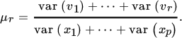
It is clear that

(2)

and hence that 0 < μ_r ≤ 1 and μ_p = 1.

Principal components analysis is only useful when, for a relatively small value of r, μ_r is close to one; in that case, a small number of principal components explains most of the variation in x.

4 A RELATED RESULT

Another way of looking at the problem of explaining the variation in x is to try and find a matrix V of specified rank r ≤ p, which provides the ‘best’ approximation of Ω. It turns out that the optimal V is a matrix whose r nonzero eigenvalues are the r largest eigenvalues of Ω.

5 SAMPLE PRINCIPAL COMPONENTS

In applied research, the variance matrix Ω is usually not known and must be estimated. To this end we consider a random sample x₁, x₂, …, x_n of size n > p from the distribution of a random p × 1 vector x. We let

where both μ and Ω are unknown (but finite). We assume that Ω is positive definite and denote its eigenvalues by λ₁ ≥ λ₂ ≥ ⋯ ≥ λ_p > 0.

The observations in the sample can be combined into the n × p observation matrix

The sample variance of x, denoted by S, is

(5)

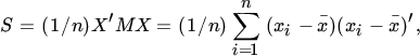
where

The sample variance is more commonly defined as S^* = (n/(n − 1))S, which has the advantage of being an unbiased estimator of Ω. We prefer to work with S as given in (5) because, given normality, it is the ML estimator of Ω.

We denote the eigenvalues of S by l₁ > l₂ > ⋯ > l_p, and notice that these are distinct with probability one even when the eigenvalues of Ω are not all distinct. Let Q = (q₁, q₂, …, q_p) be a p × p orthogonal matrix such that

We then define the p × 1 vector

as the vector of sample principal components of x, and its ith element as the ith sample principal component.

Recall that T = (t₁, …, t_p) denotes a p × p orthogonal matrix such that

We would expect that the matrices S, Q, and L from the sample provide good estimates of the corresponding population matrices Ω, T, and Λ. That this is indeed the case follows from the next theorem.

6 OPTIMALITY OF SAMPLE PRINCIPAL COMPONENTS

In direct analogy with population principal components, the sample principal components have the following optimality property.

7 ONE‐MODE COMPONENT ANALYSIS

Let X be the n × p observation matrix and M = I_n − (1/n)ιι′. As in ( 5 ), we express the sample variance matrix S as

In Theorem 17.6, we found the best approximation to S by a matrix V of given rank. Of course, instead of approximating S we can also approximate X by a matrix of given (lower) rank. This is attempted in component analysis.

In the one‐mode component model, we try to approximate the p columns of X = (x¹, …, x^p) by linear combinations of a smaller number of vectors z¹, …, z^r. In other words, we write

(6)

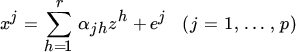
and try to make the residuals e^j ‘as small as possible’ by suitable choices of {z^h} and {α_jh}. In matrix notation, (6) becomes

(7)

The n × r matrix Z is known as the core matrix. Without loss of generality, we may assume A′A = I_r (see Exercise 1). Even with this constraint on A, there is some indeterminacy in (7). We can postmultiply Z with an orthogonal matrix R and premultiply A′ with R′ without changing ZA′ or the constraint A′A = I_r.

Let us introduce the set of matrices

This is the set of all semi‐orthogonal p × r matrices, also known as the Stiefel manifold.

With this notation we can now prove Theorem 17.7.

We notice that the ‘best’ approximation to X, say , is given by (15): . It is important to observe that is part of a singular‐value decomposition of X, namely the part corresponding to the r largest eigenvalues of X′X. To see this, assume that r(X) = p and that the eigenvalues of X′X are given by λ₁ ≥ λ₂ ≥ ⋯ ≥ λ_p > 0. Let Λ = diag(λ₁, …, λ_p) and let

(16)

be a singular‐value decomposition of X, with S′S = T′T = I_p. Let

(17)

and partition S and T accordingly as

(18)

Then,

From (16)–(18), we see that X′XT₁ = T₁Λ₁, in accordance with (13). The approximation can then be written as

This result will be helpful in the treatment of two‐mode component analysis in Section 17.9 . Notice that when r(ZA′) = r(X), then (see also Exercise 3).

8 ONE‐MODE COMPONENT ANALYSIS AND SAMPLE PRINCIPAL COMPONENTS

In the one‐mode component model we attempted to approximate the n × p matrix X by ZA′ satisfying A′A = I_r. The solution, from Theorem 17.7, is

where T₁ is a p × r matrix of eigenvectors associated with the r largest eigenvalues of X′X.

If, instead of X, we approximate MX by ZA′ under the constraint A′A = I_r, we find in precisely the same way

but now T₁ is a p × r matrix of eigenvectors associated with the r largest eigenvalues of (MX)′(MX) = X′MX. This suggests that a suitable approximation to X′MX is provided by

(19)

where Λ₁ is an r × r matrix containing the r largest eigenvalues of X′MX. Now, (19) is precisely the approximation obtained in Theorem 17.6. Thus, one‐mode component analysis and sample principal components are tightly connected.

9 TWO‐MODE COMPONENT ANALYSIS

Suppose that our data set consists of a 27 × 6 matrix X containing the scores given by n = 27 individuals to each of p = 6 television commercials. A onemode component analysis would attempt to reduce p from 6 to 2 (say). There is no reason, however, why we should not also reduce n, say from 27 to 4. This is attempted in two‐mode component analysis, where the purpose is to find matrices A, B, and Z such that

with A′A = I_r1 and B′B = I_r2, and ‘minimal’ residual matrix E. (In our example, r₁ = 2, r₂ = 4.) When r₁ = r₂, the result follows directly from Theorem 17.7 and we obtain Theorem 17.8.

In the more general case where r₁ ≠ r₂, the solution is essentially the same. A better approximation does not exist. Suppose r₂ > r₁. Then we can extend B with r₂ − r₁ additional columns such that B′B = I_r2, and we can extend Z with r₂ − r₁ additional rows of zeros. The approximation is still the same: . Adding columns to B turns out to be useless; it does not lead to a better approximation to X, since the rank of BZA′ remains r₁.

10 MULTIMODE COMPONENT ANALYSIS

Continuing our example of Section 17.9 , suppose that we now have an enlarged data set consisting of a three‐dimensional matrix X of order 27 × 6 × 5 containing scores by p₁ = 27 individuals to each of p₂ = 6 television commercials; each commercial is shown p₃ = 5 times to every individual. A three‐mode component analysis would attempt to reduce p₁, p₂, and p₃ to, say, r₁ = 6, r₂ = 2, r₃ = 3. Since, in principle, there is no limit to the number of modes we might be interested in, let us consider the s‐mode model. First, however, we reconsider the two‐mode case

(20)

We rewrite (20) as

where x = vec X, z = vec Z, and e = vec E. This suggests the following formulation for the s‐mode component case:

where A_i is a p_i × r_i matrix satisfying . The data vector x and the ‘core’ vector z can be considered as stacked versions of s‐dimensional matrices X and Z. The elements in x are identified by s indices with the ith index assuming the values 1, 2, …, p_i. The elements are arranged in such a way that the first index runs slowly and the last index runs fast. The elements in z are also identified by s indices; the ith index runs from 1 to r_i.

The mathematical problem is to choose A_i(i = 1, …, s) and z in such a way that the residual e is ‘as small as possible’.

11 FACTOR ANALYSIS

Let x be an observable p × 1 random vector with E x = μ and var(x) = Ω. The factor analysis model assumes that the observations are generated by the structure

(30)

where y is an m × 1 vector of nonobservable random variables called ‘common factors’, A is a p × m matrix of unknown parameters called ‘factor loadings’, and ɛ is a p × 1 vector of nonobservable random errors. It is assumed that y ~ N(0, I_m), ɛ ~ N(0, Φ), where Φ is diagonal positive definite, and that y and ɛ are independent. Given these assumptions, we find that x ~ N(μ, Ω) with

(31)

There is clearly a problem of identifying A from AA′, because if A^* = AT is an orthogonal transformation of A, then A^*A^*′ = AA′. We shall see later (Section 17.14 ) how this ambiguity can be resolved.

Suppose that a random sample of n > p observations x₁, …, x_n of x is obtained. The loglikelihood is

(32)

Maximizing Λ with respect to μ yields . Substituting for μ in (32) yields the so‐called concentrated loglikelihood

(33)

with

Clearly, maximizing (33) is equivalent to minimizing log |Ω| + tr Ω⁻¹ S with respect to A and Φ. The following theorem assumes Φ known, and thus minimizes with respect to A only.

Notice that the optimal choice for A is such that A′Φ⁻¹ A is a diagonal matrix, even though this was not imposed.

12 A ZIGZAG ROUTINE

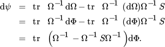
Theorem 17.10 provides the basis for (at least) two procedures by which ML estimates of A and Φ in the factor model can be found. The first procedure is to minimize the concentrated function (36) with respect to the p diagonal elements of Φ. The second procedure is based on the first‐order conditions obtained from minimizing the function

(44)

The function ψ is the same as the function ϕ defined in (34) except that ϕ is a function of A given Φ, while ψ is a function of A and Φ.

In this section, we investigate the second procedure. The first procedure is discussed in Section 17.13.

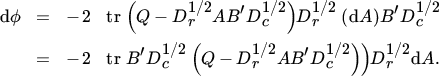
From ( 37 ), we see that the first‐order condition of ψ with respect to A is given by

(45)

where Ω = AA′ + Φ. To obtain the first‐order condition with respect to Φ, we differentiate ψ holding A constant. This yields

Since Φ is diagonal, the first‐order condition with respect to Φ is

(46)

Pre‐ and postmultiplying (46) by Φ, we obtain the equivalent condition

(47)

(The equivalence follows from the fact that Φ is diagonal and nonsingular.) Now, given the first‐order condition for A in (45), and writing Ω − AA′ for Φ, we have

so that

using the fact that ΦΩ⁻¹S = SΩ⁻¹ Φ. Hence, given ( 45 ), (47) is equivalent to

that is,

(48)

Thus, Theorem 17.10 provides an explicit solution for A as a function of Φ and (48) gives Φ as an explicit function of A. A zigzag routine suggests itself: choose an appropriate starting value for Φ, then calculate AA′ from (43), then Φ from ( 48 ), et cetera. If convergence occurs (which is not guaranteed), then the resulting values for Φ and AA′ correspond to a (local) minimum of ψ.

From ( 43 ) and ( 48 ), we summarize this iterative procedure as

for k = 0, 1, 2, ….Here s_ii denotes the ith diagonal element of S, the jth largest eigenvalue of (Φ^(k))^−1/2S(Φ^(k))^−1/2, and the corresponding eigenvector.

What is an appropriate starting value for Φ? From ( 48 ), we see that 0 < ϕ_i < s_ii (i = 1, …, p). This suggests that we choose our starting value as

for some α satisfying 0 < α < 1. Calculating A from (35) given Φ = Φ⁽⁰⁾ leads to

where Λ is a diagonal m × m matrix containing the m largest eigenvalues of S^* = (dg S)^−1/2 S(dg S)^−1/2 and T is a p × m matrix of corresponding orthonormal eigenvectors. This shows that α must be chosen smaller than each of the m largest eigenvalues of S^*.

13 NEWTON‐RAPHSON ROUTINE

Instead of using the first‐order conditions to set up a zigzag procedure, we can also use the Newton‐Raphson method in order to find the values of ϕ₁, …, ϕ_p that minimize the concentrated function ( 36 ). The Newton‐Raphson method requires knowledge of the first‐ and second‐order derivatives of this function, and these are provided by the following theorem.

Given knowledge of the gradient g(ϕ) and the Hessian G(ϕ) from (50) and (51), the Newton‐Raphson method proceeds as follows. First choose a starting value ϕ⁽⁰⁾. Then, for k = 0, 1, 2, …, compute

This method appears to work well in practice and yields the values ϕ₁, …, ϕ_p, which minimize (49). Given these values we can compute A from ( 35 ), thus completing the solution.

There is, however, one proviso. In Theorem 17.11 we require that the p − m smallest eigenvalues of Φ^−1/2 SΦ^−1/2 are all distinct. But, by rewriting (31) as

we see that the p − m smallest eigenvalues of Φ^−1/2 ΩΦ^−1/2 are all one. Therefore, if the sample size increases, the p − m smallest eigenvalues of Φ^−1/2 SΦ^−1/2 will all converge to one. For large samples, an optimization method based on Theorem 17.11 may therefore not give reliable results.

14 KAISER'S VARIMAX METHOD

The factorization Ω = AA′ + Φ of the variance matrix is not unique. If we transform the ‘loading’ matrix A by an orthogonal matrix T, then we have (AT)(AT)′ = AA′. Thus, we can always rotate A by an orthogonal matrix T, so that A^* = AT yields the same Ω. Several approaches have been suggested to use this ambiguity in a factor analysis solution in order to create maximum contrast between the columns of A. A well‐known method, due to Kaiser, is to maximize the raw varimax criterion.

Kaiser defined the simplicity of the kth factor, denoted by s_k, as the sample variance of its squared factor loadings. Thus,

(62)

The total simplicity is s = s₁ + s₂ + ⋯ + s_m and the raw varimax method selects an orthogonal matrix T such that s is maximized.

An iterative zigzag procedure can be based on (64) and ( 65 ). In ( 64 ), we have B = B(Q) and in ( 65 ) we have Q = Q(B). An obvious starting value for B is B⁽⁰⁾ = A. Then calculate Q⁽¹⁾ = Q(B⁽⁰⁾), B⁽¹⁾ = B(Q⁽¹⁾), Q⁽²⁾ = Q(B⁽¹⁾), et cetera. If the procedure converges, which is not guaranteed, then a (local) maximum of (63) has been found.

15 CANONICAL CORRELATIONS AND VARIATES IN THE POPULATION

Let z be a random vector with zero expectations and positive definite variance matrix Σ. Let z and Σ be partitioned as

(69)

so that Σ₁₁ is the variance matrix of z⁽¹⁾, Σ₂₂ the variance matrix of z⁽²⁾, and the covariance matrix between z⁽¹⁾ and z⁽²⁾.

The pair of linear combinations u′z⁽¹⁾ and v′z⁽²⁾, each of unit variance, with maximum correlation (in absolute value) is called the first pair of canonical variates and its correlation is called the first canonical correlation between z⁽¹⁾ and z⁽²⁾.

The kth pair of canonical variates is the pair u′z⁽¹⁾ and v′z⁽²⁾, each of unit variance and uncorrelated with the first k − 1 pairs of canonical variates, with maximum correlation (in absolute value). This correlation is the kth canonical correlation.

16 CORRESPONDENCE ANALYSIS

Correspondence analysis is a multivariate statistical technique, conceptually similar to principal component analysis, but applied to categorical rather than to continuous data. It provides a graphical representation of contingency tables, which arise whenever it is possible to place events into two or more categories, such as product and location for purchases in market research or symptom and treatment in medical testing. A well‐known application of correspondence analysis is textual analysis — identifying the author of a text based on examination of its characteristics.

We start with an m × n data matrix P with nonnegative elements which sum to one, that is, ι′Pι = 1, where ι denotes a vector of ones (of unspecified dimension). We let r = Pι and c = P′ι denote the vectors of row and column sums, respectively, and D_r and D_c the diagonal matrices with the components of r and c on the diagonal.

Now define the matrix

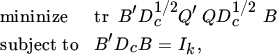
Correspondence analysis then amounts to the following approximation problem,

with respect to A and B. The dimension of the approximation is k < n.

To solve this problem, we first maximize with respect to A taking B to be given and satisfying the restriction B′D_cB = I_k. Thus, we let

from which we find

The maximum (with respect to A) is therefore obtained when

and this gives, taking the constraint B′D_cB = I_k into account,

Hence,

Our maximization problem thus becomes a minimization problem, namely

(75)

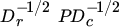
with respect to B. Now let . Then we can rewrite (75) as

with respect to X. But we know the answer to this problem, see Theorem 11.13. The minimum is the sum of the k smallest eigenvalues of Q′Q and the solution contains the k eigenvectors associated to these eigenvalues. Hence, the complete solution is given by

so that the data approximation is given by

17 LINEAR DISCRIMINANT ANALYSIS

Linear discriminant analysis is used as a signal classification tool in signal processing applications, such as speech recognition and image processing. The aim is to reduce the dimension in a such a way that the discrimination between different signal classes is maximized given a certain measure. The measure that is used to quantify the discrimination between different signal classes is the generalized Rayleigh quotient,

where A is positive semidefinite and B is positive definite.

This measure is appropriate in one dimension. If we wish to measure the discrimination between signal classes in a higher‐ (say k‐)dimensional space, we can use the k‐dimensional version of the quotient, that is,

(76)

where X is an n × k matrix of rank k, A is positive semidefinite of rank r ≥ k, and B is positive definite.

Let us define

(77)

Then,

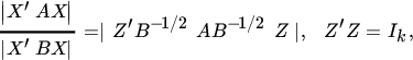
and hence, by Theorem 11.15, this is maximized at , where contains the eigenvectors associated with the k largest eigenvalues of B^−1/2AB^−1/2. The solution matrix is unique (apart from column permutations), but the resulting matrix is not unique. In fact, the class of solution matrices is given by

(78)

where Q is an arbitrary positive definite matrix. This can be seen as follows. First, it follows from (77) that 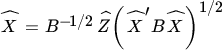, which implies (78) for . Next, suppose that (78) holds for some positive definite Q and semi‐orthogonal . Then,

so that ( 77 ) holds.

BIBLIOGRAPHICAL NOTES

1. There are some excellent texts on multivariate statistics and psychometrics; for example, Morrison (1976), Anderson (1984), Mardia, Kent, and Bibby (1992), and Adachi (2016).

2–3. See also Lawley and Maxwell (1971), Muirhead (1982), and Anderson (1984).

5–6. See Morrison (1976) and Muirhead (1982). Theorem 17.4 is proved in Anderson (1984). For asymptotic distributional results concerning l_i and q_i, see Kollo and Neudecker (1993). For asymptotic distributional results concerning q_i in Hotelling's (1933) model where , see Kollo and Neudecker (1997a).

7–9. See Eckart and Young (1936), Theil (1971), Ten Berge (1993), Greene (1993), and Chipman (1996). We are grateful to Jos Ten Berge for pointing out a redundancy in (an earlier version of) Theorem 17.8.

10. For three‐mode component analysis, see Tucker (1966). An extension to four models is given in Lastovička (1981) and to an arbitrary number of modes in Kapteyn, Neudecker, and Wansbeek (1986).

11–12. For factor analysis, see Rao (1955), Morrison (1976), and Mardia, Kent, and Bibby (1992). Kano and Ihara (1994) propose a likelihood‐based procedure for identifying a variate as inconsistent in factor analysis. Tsai and Tsay (2010) consider estimation of constrained and partially constrained factor models when the dimension of explanatory variables is high, employing both maximum likelihood and least squares. Yuan, Marshall, and Bentler (2002) extend factor analysis to missing and nonnormal data.

13. See Clarke (1970), Lawley and Maxwell (1971), and Neudecker (1975).

14. See Kaiser (1958, 1959), Sherin (1966), Lawley and Maxwell (1971), and Neudecker (1981). For a generalization of the matrix results for the raw varimax rotation, see Hayashi and Yung (1999).

15. See Muirhead (1982) and Anderson (1984).

16. Correspondence analysis is discussed in Greenacre (1984) and Nishisato (1994). The current discussion follows van de Velden, Iodice d'Enza, and Palumbo (2017). A famous exponent of textual analysis is Foster (2001), who describes how he identified the authors of several anonymous works.

17. See Duda, Hart, and Stork (2001) and Prieto (2003).