
So far, we have considered performance tuning singleton MongoDB servers – servers that are not part of a cluster. However, most production MongoDB instances are configured as replica sets, since only this configuration provides sufficient high availability guarantees for modern “always-on” applications.
None of the tuning principles we have covered in previous chapters are invalidated in a replica set configuration. However, replica sets provide us with some additional performance challenges and opportunities which are covered in this chapter.
MongoDB Atlas provides us with an easy way to create cloud-hosted, fully managed MongoDB clusters. As well as offering convenience and economic advantages, MongoDB Atlas contains some unique features that involve performance opportunities and challenges.
Replica Set Fundamentals
We introduced replica sets in Chapter 2. A replica set following best practice consists of a primary node together with two or more secondary nodes. It is recommended to use three or more nodes, with an odd number of total nodes. The primary node accepts all write requests which are propagated synchronously or asynchronously to the secondary nodes. In the event of a failure of a primary, an election occurs to which a secondary node is elected to serve as the new primary and database operations can continue.
In a default configuration, the performance impact of a replica set is minimal. All read and write operations will be directed to the primary, and while there will be a small overhead incurred by the primary in transmitting data to secondaries, this overhead is rarely critical.
However, if a higher degree of fault tolerance is required, then write performance can be sacrificed by requiring writes to complete on one or more secondaries before being confirmed. This is controlled by the MongoDB write concern parameter. Additionally, the MongoDB read preference parameter can be configured to allow secondaries to service read requests, potentially improving read performance.
In order to clearly illustrate the relative effects of read preference and write concern, we've used a replica set with widely geographically distributed nodes – in Hong Kong, Seoul, and Tokyo, with application workloads originating in Sydney. This configuration has much higher latencies than are typical but allows us to show the relative effects of various configurations more clearly.
Using Read Preference
The secondary nodes are likely to be less busy than the primary and, therefore, able to respond more quickly to read requests.
By directing reads to secondary nodes, we reduce load on the primary, possibly increasing the write throughput of the cluster.
By spreading read requests across all the nodes of the cluster, we improve overall read throughput since we are taking advantage of the otherwise idle secondaries.
We might be able to reduce network latency by directing read requests to a secondary which is “nearer” to us – in terms of network latency.
These advantages need to be balanced against the possibility of reading “stale” data. In a default configuration, only the master is guaranteed to have up-to-date copies of all information (though we can change this by adjusting write concern as described in the next section). If we read from a secondary, we might get out-of-date information.
Secondary reads may result in stale data being returned. If this is unacceptable, either configure write concern to prevent stale reads or use the default primary read concern.
Read preference settings
Read Preference | Effect |
|---|---|
primary | This is the default. All reads are directed to the replica set primary. |
primaryPreferred | Direct reads to the primary, but if no primary is available, direct reads to a secondary. |
secondary | Direct reads to a secondary. |
secondaryPreferred | Direct reads to a secondary, but if no secondary is available, direct reads to the primary. |
nearest | Direct reads to the replica set member with the lowest network round trip time to the calling program. |
If you have decided to route reads to a non-primary node, secondaryPreferred or nearest are the recommended settings. secondaryPreferred is generally better than secondary, because it allows reads to fall back to the primary if no secondaries are available. When there are multiple secondaries to choose from and some are “further away” (have greater network latencies), then nearest will route requests to the “closest” node – secondary or non-secondary.

Effect of read preference on read performance (reading 411,000 documents)
Secondary reads will usually be faster than primary reads. The nearest read preference can help pick the replica set node with the lowest network latency.
Setting Read Preference
Read preference can be set at the connection level or at the statement level.
See your MongoDB driver documentation for guidance in setting read preference in your programming language.
maxStalenessSeconds
maxStalenessSeconds can be added to a read preference to control the tolerable lag in data. When picking a secondary node, the MongoDB driver will only consider those nodes who have data within maxStalenessSeconds seconds of the primary. The minimum value is 90 seconds.
maxStalenessSeconds can protect you from seriously out-of-date data when using secondary read preferences.
Tag Sets
Tag sets can be used to fine-tune read preference. Using tag sets, we can direct queries to specific secondaries or sets of secondaries. For instance, we could nominate a node as a business intelligence server and another node for web application traffic.
If we want to set up a specific secondary as a read-only server for analytics, tag sets are a perfect solution.
We can also use tag sets to distribute workload evenly across the nodes in a server. For instance, consider a scenario in which we are reading data from three collections in parallel. With the default read preference, all the reads will be directed to the primary. If we choose secondaryPreferred, then we might get more nodes participating in the work, but it’s still possible that all the requests will go to the same node. However, with tag sets, we can direct each query to a different node.
Queries against collections iotData2 and iotData3 could similarly be directed to Korea and Japan. Not only does this allow every node in the cluster to participate simultaneously, it also helps with cache effectiveness – since each node is responsible for a specific collection, all of that node’s cache can be dedicated to that collection.

Using tag sets to distribute work across all nodes in a cluster
Tag sets can be used to direct read requests to specific nodes. You can use tag sets to nominate nodes for special purposes such as analytics or to distribute read workload more evenly across all nodes in the cluster.
Write Concern
Read preference helps MongoDB decide which server should service a read request. Write concern tells MongoDB how many servers should be involved in a write request.
w controls how many nodes should receive the write before the write operation can complete. w can be set to a number or to “majority”.
j controls whether write operations require a journal write before completing. It is set to true or false.
wtimeout specifies the amount of time allowed to achieve the write concern before returning an error.
Journaling
If j:false is specified, then a write is considered complete provided it is received by the mongod server. If j:true is specified, then the write is considered complete once it is written to the write-ahead journal that we discussed in Chapter 12.
Running without journaling is considered reckless since it allows for a loss of data if the mongod server crashes. However, some configurations allow for such data loss anyway. For instance, in a w:1,j:true scenario, data might be lost if a server dies and fails over to a secondary which has not yet received the write. In this case, setting j:false might give an increase in throughput without an unacceptable increase in the chance of data loss.
The Write Concern w Option
The w option controls how many nodes in the cluster must receive a write before the write operation completes. The default setting of 1 requires that only the primary receives the write. Higher values require the write to propagate to a larger number of nodes.
The w:"majority" setting requires that a majority of nodes receive the write operation before the write completes. w:"majority" is a sensible default for systems in which data loss is deemed unacceptable. If the majority of nodes have the update, then in any single-node failure or network partition scenario, the newly elected primary will have access to that data.
Of course, the impact of writing to multiple nodes has a performance overhead. You might imagine that your data is being written to multiple nodes simultaneously. However, the write is made to the primary and only then propagated to the other nodes through the replication mechanism. If there is already a significant replication lag, then the delay may be much higher than expected. Even if the replication lag is minimal, the replication can only commence after the initial write has succeeded, so the performance lag is always greater than w:1.

Sequence of events for w:2, j:true write concern

Effect of write concern on write throughput
Your setting for write concern should be determined by fault tolerance concerns, not by write performance. However, it’s important to realize that higher levels of write concern have potentially significant performance impacts.
Higher levels of write concern can result in a significant slowdown in write throughput. However, lower levels of write concern may result in data loss in the event of server failure.
As we can see, w:0 provides the absolute best performance. However, a write with w:0 can succeed even if the data doesn’t make it to the MongoDB server. Even a transitory network failure might result in a loss of data. In almost all circumstances, w:0 is just too unreliable.
A write concern of w:0 might result in a performance boost, but at the cost of completely unreliable data writes.
Write Concern and Secondary Reads
Although higher levels of write concern slow down modification workloads, there may be a pleasant side effect if your overall application performance is read-dominated. If the write concern is set to write to all members of the cluster, then secondary reads will always return the correct data. This might allow you to use secondary reads even if you cannot tolerate stale queries.
However, be aware that if you manually set the write concern the number of nodes in the cluster, any failures in the cluster may result in reads timing out.
Setting w to the number of nodes in the cluster will result in secondary reads always returning up-to-date data. However, write operations might fail if a node is unavailable.
MongoDB Atlas
MongoDB Atlas is MongoDB’s fully managed database-as-a-service (DBaaS) offering. Using Atlas, you can create and configure MongoDB replica sets and sharded clusters from a web interface without having to configure your own hardware or virtual machines. Atlas takes care of most of database operational considerations including backups, version upgrades, and performance monitoring. Atlas is also available in the three major public clouds: AWS, Azure, and Google Cloud.
When it comes to deploying a MongoDB cluster, Atlas offers a lot of convenience by handling much of the dirty work behind the scenes. However, as well as the operational advantages, Atlas boasts additional features not available for other deployment types. These features include advanced sharding and query options that can be highly appealing when creating a new cluster.
Although implementing these options may be as simple as clicking a button, it is essential to remember that they can also require careful planning and design to meet their full potential. In the following, we will go through a number of these Atlas features along with their performance implications.
Atlas Search
Atlas Search (formerly known as Atlas Full-Text Search ) is a feature built upon Apache Lucene to provide a more powerful text search functionality. Although all versions of MongoDB support text indexes (see Chapter 5), the Apache Lucene integration provides far more powerful text search capabilities.
The strength of Apache Lucene is provided through analyzers. Simply put, analyzers will determine how your text index is created. You can create a custom analyzer, but Atlas provides built-in options that will cover the majority of use cases.
Choosing an appropriate analyzer during index creation is one of the easiest ways to improve the results of your Atlas Search queries.
When we talk about improving the performance of text search, we are not always referring to query speed. Some analyzers may improve the "performance" of a query by providing more relevant scoring results, but may also lead to slower queries.
Standard: All words are converted to lowercase and punctuation is ignored. Additionally, the standard analyzer can correctly interpret special symbols and acronyms and will discard joining words like “and” to provide better results. The standard analyzer creates index entries for each “word” and is the most commonly useful index type.
Simple: As you might guess, the simple analyzer is like the standard analyzer but with less advanced logic when determining a “word” for each index entry. All words are converted to lowercase. A simple analyzer will create an entry by finding a word between any two characters that are not a letter. Unlike the standard analyzer, the simple analyzer will not handle joining words.
Whitespace: If the simple analyzer is a dumbed-down version of the standard analyzer, the whitespace analyzer takes this even further. Words will not be converted to lowercase, and entries are created for any string divided by a whitespace character with no additional handling of punctuation or special characters.
Keyword: The keyword analyzer takes the entire value of the field as a single entry, requiring exact matches to return the result in a query. This is the most specific analyzer provided.
Language: The language analyzer is where Lucene is particularly powerful, as it provides a series of presets for each language you might encounter. Each preset will create index entries based on the typical structure of text written in that language.
When creating Atlas Search indexes, there is no single best analyzer to choose, and making a choice will not be about query speed alone. You will have to consider the shape of your data and the type of queries users are likely to send.
Let’s look at an example based upon a property rental marketplace dataset. In this dataset, large amounts of text data exist in various attributes. Names, addresses, descriptions, and property metadata are all stored as strings for each listing, along with reviews and comments.
Each of these attributes is best suited to different types of search indexes based on which analyzer most fits the matching query. Descriptions and comments may best be served by a language index which interprets language-specific semantics. Property types like “house” or “apartment” match a keyword analyzer best as we want exact matches. Other fields are probably indexed correctly by the standard analyzer or may not need indexing at all.

Index size by analyzer and field length (5555 documents)
Although these results will vary greatly depending on the text data itself, this chart primarily indicates two things.
Firstly, a smaller text field will produce little to no variation in index size (and thus the time taken to scan that index). This makes sense, since a smaller number of words or characters can be subdivided into a smaller number of ways and are less likely to require complex rules to create the index.
Secondly, on larger, more complex text data, the size of the index can vary significantly between analyzer types. Sometimes a larger index will be a good thing, providing superior results and performance. However, it’s still something worth considering when creating Atlas Search indexes.

Query duration by index analyzer type (5555 documents, 1000 queries)
If we were to look at this data alone, we would assume that the keyword analyzer will provide us with the best performance for our query. However, with any text search, we also need to take into account the scoring of our results.
Performance of different analyzer types
Analyzer | Query Time (min) | Score | Document |
|---|---|---|---|
Standard | 2.13 | 6.25 | Studio 1 Q Leblon, Promo de… |
Simple | 2.50 | 6.09 | Studio 1 Q Leblon, Promo de... |
Whitespace | 2.10 | 6.16 | Tree Fern Garden Appt,… |
Keyword | 1.99 | ||
Language | 2.11 | 5.48 | Studio 1 Q Leblon, Promo de... |
The first thing you may notice is that the keyword analyzer returned no documents (and thus a 0 score) for our query, despite having the lowest query time. This is expected, as the keyword index requires an exact match to the entire value of the field. So although it’s fast, it doesn’t necessarily return the best results.
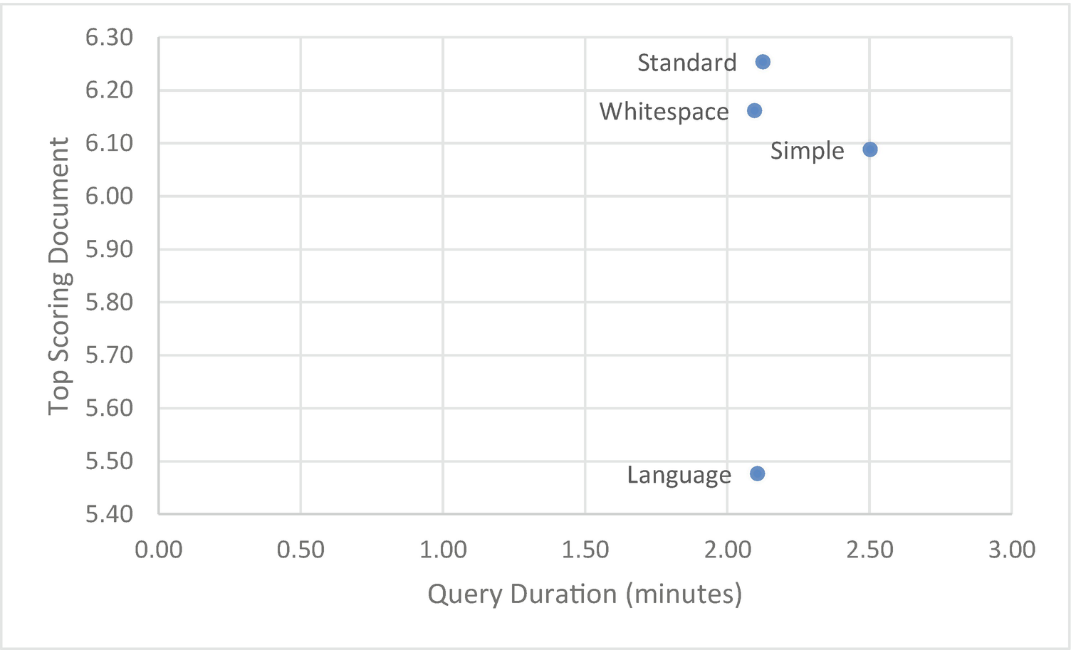
Query duration, document score, and document by analyzer (5555 documents, 1000 queries)
These results correspond roughly to our created index size, with the larger indexes taking longer to return a result. Interestingly, although the standard analyzer is not the quickest, it does provide the best combination of high confidence results for only a fraction more query time. You may have expected a language-specific analyzer to perform better than the standard analyzer. In this case, there are multiple languages both in the indexed field and across many other fields. When it comes to user input, it’s hard to guarantee a single unified language.
You could repeat this analysis on your dataset to try and find the right analyzer for your Atlas Search. It is integral to think about the type of data, as well as the types of queries when creating an Atlas Search index. Although there is no always-right or always-wrong answer, the standard analyzer is likely to provide you with good overall performance. However, be aware that different analyzers can return different results, and it’s generally not good practice to make a query faster if doing so returns the wrong results.
The various Atlas Search text search analyzers have different performance characteristics. However, the fastest analyzer might not return the best results for your application. Make sure you balance the accuracy of results with the speed of the text search.
Atlas Data Lake
The concept of a “Data Lake” as a centralized repository of large amounts of structured or unstructured data became popular with the rise of Big Data and technologies like Hadoop. Since then, it has become a standard fixture in many enterprise environments. MongoDB introduced Atlas Data Lake as a method to integrate with this pattern. In a nutshell, the Atlas Data Lake allows you to query data from an Amazon S3 bucket using the Mongo Query Language.
Atlas Data Lake is a powerful tool for extending the reach of your MongoDB system to external, non-BSON data, and although it has the look and feel of a normal MongoDB database, there are some considerations to take into account when querying Data Lake.
The first aspect of Data Lake that may stop you in your tracks is the lack of indexes. There are no indexes in Data Lake, so by default, many of your queries will be resolved by a complete scan of all files.
However, there is a way around this limitation. By creating files whose names reflect a key attribute value, we can restrict the file accesses to only relevant files.
We can see that only a single file (partition) was accessed along with the name of the matching partition.
We can avoid having to scan all files in an Atlas Data Lake by creating files whose contents and file names correspond to a particular key value.
Another area where a lack of indexes can cause problems is in the case of $lookup. As we discussed in Chapter 7, indexes are absolutely essential when optimizing joins with $lookup.

$lookup performance by file structure in Data Lake (5555 documents)
Additionally, this method is far more scalable. With a $lookup against a single file, the file must be repeatedly scanned for each customer we join. However, with separate files for each customer, a much smaller file is read for each $lookup operation. With a single large file, performance will steeply degrade as documents are added to the file, whereas with multiple files, performance will scale more linearly.
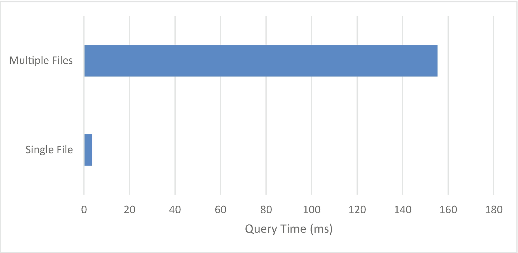
Full collection query duration by file structure in Data Lake (254,058 documents)
In summary, while you can’t index files directly in Data Lake, you can make up for some of the lost performance by manipulating file names. The file name can become a sort of high-level index, which is particularly useful when using $lookup. However, if you are always accessing the complete dataset, your scan performance will be best on a single file.
Summary
Most MongoDB production implementations incorporate replica sets to provide high availability and fault tolerance. Replica sets are not intended to solve performance problems, but they definitely have performance implications.
In a replica set, read preference can be set to allow reads from secondary nodes. Secondary reads can distribute work across more nodes in the cluster, reduce network latency in geographically distributed clusters, and allow for parallel processing of workloads. However, secondary reads can return out-of-date results which won’t always be acceptable.
Replica set write concern controls how many nodes must acknowledge a write before the write can be acknowledged. Higher levels of write concern provide greater guarantees around data, but at the expense of performance.
MongoDB Atlas adds at least two significant features that have performance implications. Atlas text search allows for more sophisticated full-text indexing, while the Atlas Data Lake allows for queries against data held on low-cost cloud storage.