In this chapter, we describe basic elements to create and plot functions of the form f (x, y).
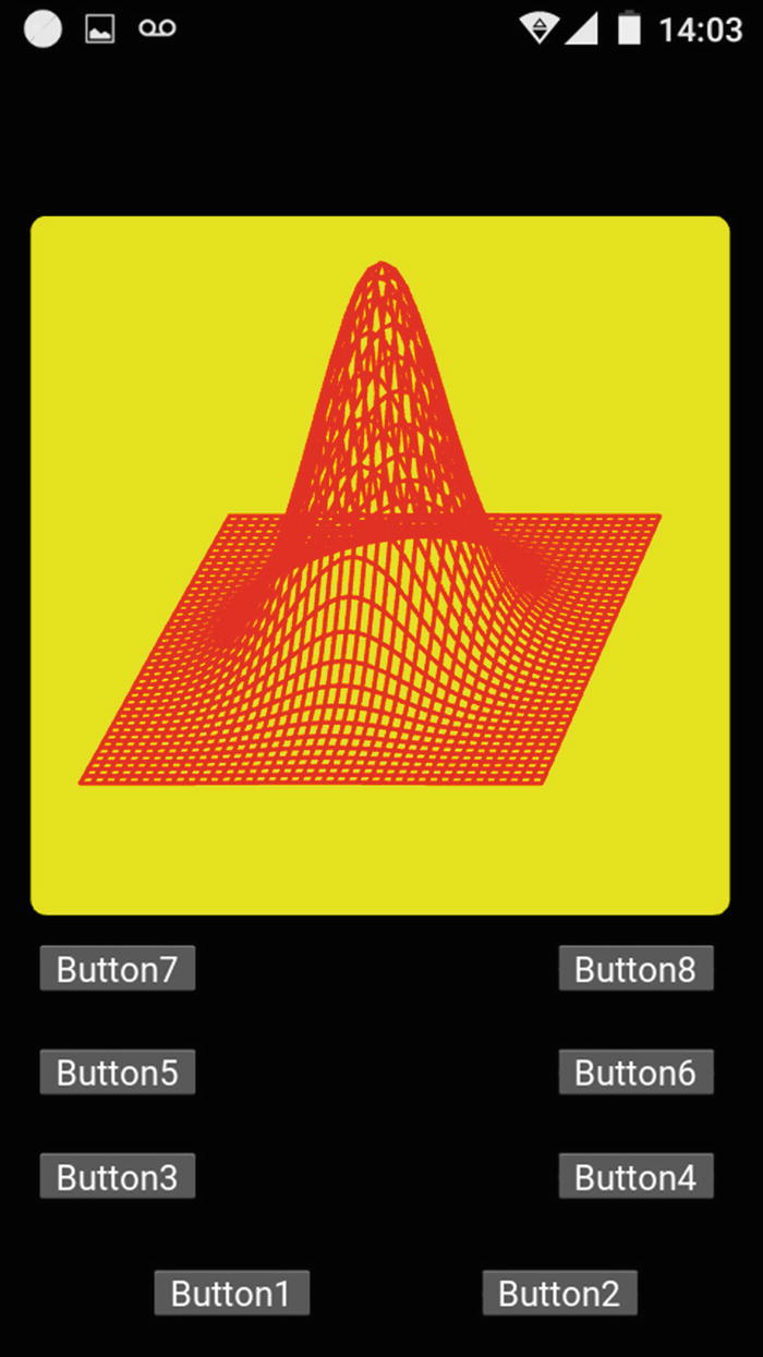
Screenshot showing a 3D plot of a circular Gaussian function
7.1 Programming the Basic Operations
The buttons in Figure 7-1 are used as follows.
Button1 shows the plot and Button2 clears the screen. Button3, Button5, and Button7 rotate and show the plot in a counterclockwise direction in steps of 5 degrees in the x-y, x-z, and y-z directions, respectively. Accordingly, Button4, Button6, and Button8 rotate the plot in clockwise directions.
In general, cell phones have limited speed capacities compared with computers. As a consequence, it is advisable to carefully press one of the buttons once and wait until the corresponding step completes.
7.2 Function Overview

In Equation (7.1), A is the amplitude (or maximum vertical height) of the Gaussian function. The x0 and y0 parameters are used to shift the function from the origin. The r0 parameter gives the semi-width of the function.
To display the plot in the screen, we need to take into account that the z-axis is normal to the screen, whereas the x- and y-axes are parallel to the screen. This is depicted in Figure 4-1, Chapter 4. Therefore, the vertical height distribution, given by f (x, y) in Equation (7.1), must be rewritten as y(x, z). This lets the y-coordinate take the roll of the vertical distribution function and the x- and z-coordinates take the roll of the horizontal and depth axes, respectively.
7.3 Generating the Axes, the Mesh, and the Function
To represent the function, it is convenient to start selecting an appropriate number of pixels, N. When setting this value, we must keep in mind that increasing N increases the precision of the plot at the cost of increasing the processing time. Conversely, decreasing N reduces the processing time, but lowers the accuracy of the results. Since we are dealing with three-dimensional data, a slight increment of N will only slightly improve the quality of the plots, but will drastically increase the processing time. According to our experience with the circular Gaussian function case, suitable graphs and processing times can be obtained when N ranges between 40 and 70.
In this code, L represents the width of the plot and D is the distance between the plane of projection and the screen. Note that in the for loop, the (n-N/2)/N*L equation will generate the x-axis ranging from -L/2 to L/2. In the for loop, when n equals 0, x[0] takes the value -L/2. At the other end, when n is N, x[N] takes the value L/2. Similarly, the z-axis ranges from -L/2 +D/2 to L/2 +D/2. This way, the z-axis represents an interval of length L, centered at D/2. These values will allow us to calculate the Gaussian function in the center of the screen and at a depth equal to D/2. This depth corresponds to the center point located between the plane of projection and the screen, as described in Chapter 6.
Note from this code that the amplitude (vertical height) of the Gaussian function is 1. The function is centered at x and z equal to 0.
Creating and Filling the Mesh and the Vertical Coordinate
Arrays x1[n][m], y1[n][m], and z1[n][m] compose the mesh. All the arrays have sizes equal to that of y[n][m], which means a unique function value can be assigned to each point in the x-z plane. This condition is necessary to allow us to rotate the three-dimensional set of points represented by the function at the corresponding (x, z) values.
7.4 Plotting the Function on the Screen
To plot the function, we need values for D, VX, VY, VZ, and N as well as x1, y, and z1.
The Factor0 parameter is used to position the function in the center of the screen.
Code for Recording the Horizontal Lines in the PointList Array
This process is repeated for the vertical lines.
GraphFunction(B) is in charge of drawing the plot. The parameter B is a handle to give us access to the widgets defined in File.kv.
Code for GraphFunction(B)
7.5 Rotating the Plot
Code for RotateFunction(B, Sense)
Code for the main.py File
Code for the File.kv File

Code for Filling y[n][m]

Plot of a Gaussian function multiplied by x, obtained using this program
7.6 Summary
In this chapter, we described basic elements to create and plot functions of the form f (x, y). You learned how to generate the axes, the mesh, and the functions. You also learned how to rotate them and display them on the screen.