12.1 Overview of Spherical Coordinates

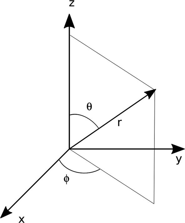
Figure 12-2 depicts a typical three-dimensional spherical-coordinate system.

In Figure 12-2, the parameters θ and ϕ represent the zenithal or polar and azimuthal angular coordinates, respectively. To generate points over a complete sphere, we need 0 < θ < π and 0 < ϕ < 2π. The r parameter is referred to as the radial distance.

From Figure 12-2, the coordinates of a point can be written as follows:

(12.1)

(12.2)

(12.3)

Equations (12.1)-(12.3) will be used to transform a three-dimensional differential equation from Cartesian coordinates into spherical coordinates.

In the following section, we present our working example, which consists of solving the well-known Schrödinger’s differential equation expressed in spherical coordinates.

12.2 Spherical Differential Equation Working Example

Consider the three-dimensional Schrödinger’s differential equation in Cartesian coordinates :

(12.4)

In Equation (12.4), the ψ(x, y, z) function will represent, in principle, all the possible spatial positions that a charged particle, with charge q and mass M, can take under the influence of a potential distribution function equal to . The term ℏ is the well-known Plank’s constant . The parameter ϵ₀ represents vacuum permittivity.

By using Equations (12.1)-(12.3), we can express Equation (12.4) in spherical coordinates, as follows:

(12.5)

Analogous to Equation (12.4), ψ(r, θ, ϕ) in Equation (12.5) gives valid spatial positions expressed in spherical coordinates for a particle with energy E, charge q, and mass M in a hydrogen-like atom with attractive potential equal to q/r.

Equation (12.5) can be solved using the method of separation of variables, proposing a solution of the product of three functions, as follows:

(12.6)

For our example, we will focus on the case r equal to a constant. Therefore, ψ(r, θ, ϕ) becomes a function of only θ and ϕ. This condition will permit us to focus on the orbitals that the electrons follow in hydrogen-like atoms. These orbitals correspond to spherical-harmonics functions, defined as follows:

(12.7)

In Equation (12.7), the square root is a normalization factor.

The atomic orbitals correspond to probabilistic spatial distributions, which analytically correspond to the square of the absolute real value of the harmonics functions, expressed as follows:

(12.8)

To plot Equation (12.8) for a set of different l, m values, we need to calculate P_{l, m}(θ, ϕ). In the following section, we focus on this subject. For illustrative purposes, the normalization factor will not be considered.

12.3 The Associated Legendre Polynomials

It can be analytically demonstrated that the associated Legendre polynomials can be generated using the following equation:

(12.9)

In Equation (12.9), we used the change of variable, x =  cos (θ). The l! expression represents the factorial of the integer l, calculated by the following expression, l!= l(l − 1)(l − 2)⋯(1).

In this code, x=sp.symbols("x") declares the variable x as symbolic, as described in Chapter 11. As a consequence, as Plm(l,m) function uses this variable for symbolic calculations, the function itself is, in turn a symbolic function.

The R=sp.lambdify( x, Plm(L_Num,M_Num) ) directive assigns to l, the value L_Num and m, the value M_NUM, respectively, 3 and 2 in this example. After executing sp.lambdify, we obtain the numerical function R(x).

Listing 12-3 gives some associated Legendre polynomials obtained with the code in Listing 12-2. When required, we have replaced rational exponents with their equivalent fractions.

P_{0, 0}(x) = 1;

Listing 12-3

List of Some Associated Legendre Polynomials

In this code, we generate the arrays Theta and Phi, each with 41 entries. The first array holds numbers ranging from 0 to π in equally spaced steps. The second array stores numbers from 0 to 2π. The first entry, called Theta[0], is equal to 0, while the last entry, Theta[40], is equal to π. In turn, Phi[0] is equal to 0 and Phi[40] is 2π.

We can verify that both methods give the same results by comparing some values.

We are now in the position of plotting some spherical harmonics functions. In the following section, we describe our method for plotting the orbitals given in Equation (12.8).

12.4 Plotting Functions in Spherical Coordinates

The program generates the associated Legendre polynomials using the code shown in Listing 12-1, which creates the numerical function R(x) to provide the associated Legendre polynomials, P_{l, m}(x).

The Factor0 variable is used to shift the plot to the center of the screen.

The code creates two arrays, each with 41 entries for the angular variables with 0 < θ < π and 0 < ϕ < 2π.

In this code, the F=np.zeros( (N+1,N+1) ) directive creates the variable F, representing a two-dimensional (N+1)*(N+1) array to store the absolute square real values of Y_{l. m}(θ, ϕ).

Now, we will use Equations (12.1)-(12.3) to create the plot. In these equations, the radial distance r is considered constant.

In this code, we included a scale factor L for enlarging or shrinking the plot as required. Finally, GraphFunction(B) and RotateFunction(B, Sense) are in charge of plotting and rotating the function, similarly to the previous chapters.

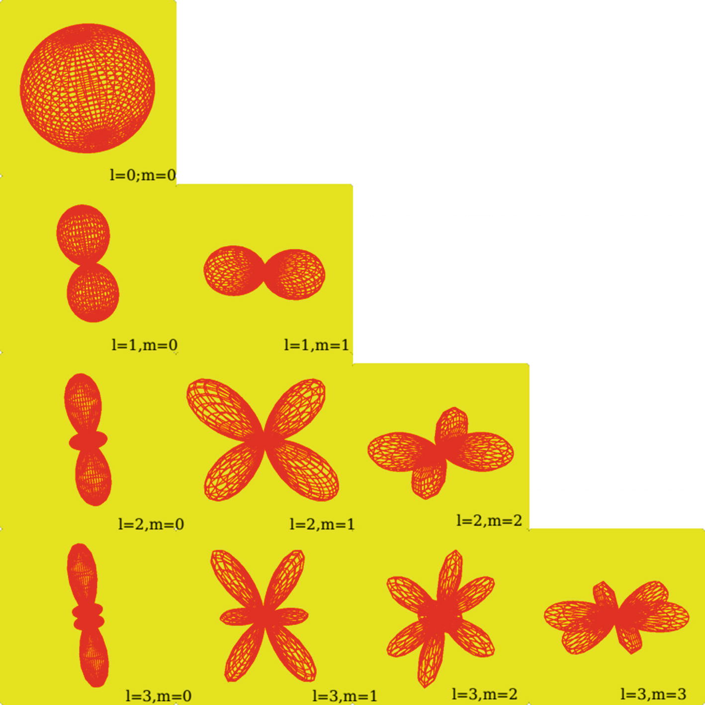
Using this code, we generated the plots of |P_{l, m}(cos(θ)) cos (mϕ)|² shown in Figure 12-3.

12.5 Summary

In this chapter, we introduced elements for plotting functions in spherical coordinates. We introduced analytical concepts on three-dimensional spherical coordinates and illustrated the programming methods with working examples of spherical harmonics polynomials.