
7
Generalization of the Classic Approach to Dealing with Uncertainty of Information and General Scheme of Multicriteria Decision‐Making under Conditions of Uncertainty
This chapter deals with multicriteria decision‐making problems under conditions of uncertainty. One of its main contributions is the consideration of choice criteria of the classic approach to handle information uncertainty in monocriteria decision‐making as objective functions within the framework of multiobjective models. Such consideration of choice criteria is of a fundamental character and allows one to modify the generalization, proposed and discussed in Ekel et al. (2008, 2011) and Pedrycz et al. (2011), of the classic approach to handle information uncertainty for solving multicriteria problems. The modification is helpful in overcoming limitations of the indicated generalization (which can lead to contradictory decisions) and chart a general methodology for multicriteria decision‐making under conditions of uncertainty. This methodology is based on a possibilistic approach to produce solutions, including robust solutions, in multicriteria analysis. Its usage, in the original form, is instrumental in using available quantitative information to the highest extent to reduce the decision uncertainty regions. If the solving capacity related to quantitative information processing does not permit one to obtain unique solutions, the methodology assumes the use, at the final decision stage, of qualitative information based on knowledge, experience, and intuition of experts involved in the decision‐making process, in particular, within the framework of <X, R> models. Thus, the general scheme is based on combining <X, F> models, <X, R> models, and the generalization of the classic approach to dealing with uncertainty of information.
However, increasingly, we encounter problems whose essence requires the consideration of the objectives (investment attractiveness, political effect, maintenance flexibility, etc.) formed on the basis of qualitative information, at all decision process stages. Considering this, the chapter describes the general scheme of multicriteria decision‐making under conditions of uncertainty aimed at generating multicriteria solutions, including multicriteria robust solutions, by constructing representative combinations of initial data, states of nature, or scenarios with direct using qualitative information (with the possibility for experts to apply diverse preference formats processed by transformation functions) presented along with quantitative information, realizing a process of information fusion within the multiobjective models.
The use of the presented results is illustrated by solving problems coming from the strategic planning area.
7.1 Generalization of the Classic Approach to Dealing with Uncertainty of Information in Multicriteria Decision Problems
As discussed in Chapter 4, the application of the Bellman–Zadeh approach (Bellman and Zadeh 1970) to decision‐making in a fuzzy environment when analyzing multicriteria models provides constructive means to derive harmonious solutions on the basis of analyzing associated maxmin problems. This circumstance permits one to propose the generalization of the classic approach to deal with information uncertainty by applying the Bellman–Zadeh approach to decision‐making in a fuzzy environment (Ekel et al. 2008, 2011; Pedrycz et al. 2011).
The results of Ekel et al. (2008, 2011) and Pedrycz et al. (2011) are related to analyzing payoff matrices, whose construction was discussed in Chapter 6. Naturally, if the considered problem includes q objective functions, then q payoff matrices are to be constructed and analyzed.
Applying Eq. (4.31) to minimized objective functions or Eq. (4.32) to maximized ones, one constructs the normalized or modified payoff matrix for the pth objective function. This payoff matrix is presented in Table 7.1.
The availability of q modified payoff matrices helps us to construct the aggregated payoff matrix presented in Table 7.2 by applying Eq. (4.28).
Table 7.1 Modified payoff matrix for the pth objective function.
| Y1 | ⋯ | Ys | ⋯ | YS | |
| X1 | ⋯ | ⋯ | |||
| ⋯ | ⋯ | ⋯ | ⋯ | ⋯ | ⋯ |
| Xk | ⋯ | ⋯ | |||
| ⋯ | ⋯ | ⋯ | ⋯ | ⋯ | ⋯ |
| XK | ⋯ | ⋯ |
Table 7.2 Aggregated payoff matrix with characteristic estimates.
| Y1 | ⋯ | Ys | ⋯ | YS | rmax(Xk) | ||||
| X1 | μD(X1, Y1) | ⋯ | μD(X1, Ys) | ⋯ | μD(X1, YS) | rmax(X1) | |||
| ⋯ | ⋯ | ⋯ | ⋯ | ⋯ | ⋯ | ⋯ | ⋯ | ⋯ | ⋯ |
| Xk | μD(Xk, Y1) | ⋯ | μD(Xk, Ys) | ⋯ | μD(Xk, YS) | rmax(Xk) | |||
| ⋯ | ⋯ | ⋯ | ⋯ | ⋯ | ⋯ | ⋯ | ⋯ | ⋯ | ⋯ |
| XK | μD(XK, Y1) | ⋯ | μD(XK, Ys) | ⋯ | μD(XK, YS) | rmax(XK) | |||
| ⋯ | ⋯ |
The characteristic estimates of Table 7.2 are the following:
- The membership function maximum level (optimistic estimate)
(7.1)
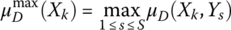
- The membership function minimum level (corresponding to the pessimistic estimate)
(7.2)

- The membership function average level
(7.3)

- The risk maximum level, which is defined as Eq. (6.4) with
 where
where  .
.
In this case, it is possible to construct the aggregated risk matrix (similar to the risk matrix given in Table 6.3) as well. One observes that if the risk matrices constructed for each objective function reflect the particular risks (monocriteria risk estimates), the aggregated risk matrix reflects the aggregated risks (multicriteria risk) in decision‐making (Pedrycz et al. 2011).
The characteristic estimates ![]() ,
, ![]() ,
, ![]() , and
, and ![]() considered here can serve as the basis for the modified choice criteria that are to be used under the generalization of the classic approach (Ekel et al. 2008, 2011; Pedrycz et al. 2011).
considered here can serve as the basis for the modified choice criteria that are to be used under the generalization of the classic approach (Ekel et al. 2008, 2011; Pedrycz et al. 2011).
In particular, the modified Wald criterion assumes the following form:
The modified Laplace criterion can be presented as follows:
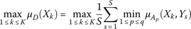
The modified Savage criterion comes in the following form:

Finally, the Hurwicz criterion takes on this form:

Although the generalization of the classic approach (Luce and Raiffa 1957; Raiffa 1968; Webster 2003) to consider the uncertainty of information in multicriteria decision‐making is concerned here with the modification of the criteria of Wald, Laplace, Savage, and Hurwicz, the same line of thought can be extended to other types of choice criteria being encountered in the literature. For instance, it is possible to apply the criteria of Hodges and Lehmann, Bayes, maximal probability, and so on (Hodges and Lehmann 1952; Trukhaev 1981). However, the use of these criteria presumes the availability of the certain type of information (usually coming in a probabilistic form) about the representative combination of initial data states of nature or scenarios.
Assuming that both criteria have to be maximized, we can apply Eq. (4.32) to build the modified payoff matrices. Tables 7.5 and 7.6 include the modified payoff matrices for the first criterion and second criterion, respectively.
Table 7.3 Example 7.1: Payoff matrix for the first criterion.
| Y1 | Y2 | Y3 | Y4 | |
| X1 | 14 | 15 | 11 | 16 |
| X2 | 9 | 11 | 13 | 14 |
| X3 | 11 | 15 | 10 | 12 |
| X4 | 16 | 13 | 12 | 14 |
Table 7.4 Example 7.1: Payoff matrix for the second criterion.
| Y1 | Y2 | Y3 | Y4 | |
| X1 | 48 | 44 | 38 | 46 |
| X2 | 43 | 38 | 39 | 47 |
| X3 | 46 | 40 | 38 | 37 |
| X4 | 40 | 38 | 39 | 45 |
Table 7.5 Example 7.1: Modified payoff matrix for the first criterion.
| Y1 | Y2 | Y3 | Y4 | |
| X1 | 0.71 | 0.86 | 0.29 | 1 |
| X2 | 0 | 0.29 | 0.57 | 0.71 |
| X3 | 0.29 | 0.86 | 0.14 | 0.43 |
| X4 | 1 | 0.57 | 0.43 | 0.71 |
Table 7.6 Example 7.1: Modified payoff matrix for the second criterion.
| Y1 | Y2 | Y3 | Y4 | |
| X1 | 1 | 0.64 | 0.09 | 0.82 |
| X2 | 0.55 | 0.09 | 0.18 | 0.91 |
| X3 | 0.82 | 0.27 | 0.09 | 0 |
| X4 | 0.27 | 0.09 | 0.18 | 0.73 |
Table 7.7 Example 7.1: Aggregated payoff matrix.
| Y1 | Y2 | Y3 | Y4 | |
| X1 | 0.71 | 0.64 | 0.09 | 0.82 |
| X2 | 0 | 0.09 | 0.18 | 0.71 |
| X3 | 0.29 | 0.27 | 0.09 | 0 |
| X4 | 0.27 | 0.09 | 0.18 | 0.71 |
The application of Eq. (4.28) permits one to build the aggregated payoff matrix, which is presented in Table 7.7. The use of Eq. (6.7) to process data of Table 7.7 leads to the aggregated risk matrix given in Table 7.8.
Table 7.8 Example 7.1: Aggregated risk matrix.
| Y1 | Y2 | Y3 | Y4 | |
| X1 | 0 | 0 | 0.09 | 0 |
| X2 | 0.71 | 0.55 | 0 | 0.11 |
| X3 | 0.42 | 0.37 | 0.09 | 0.82 |
| X4 | 0.44 | 0.55 | 0 | 0.11 |
Table 7.9 Example 7.1: Aggregated payoff matrix with characteristic estimates.
| Y1 | Y2 | Y3 | Y4 | rmax(Xk) | ||||
| X1 | 0.71 | 0.64 | 0.09 | 0.82 | 0.82 | 0.09 | 0.57 | 0.09 |
| X2 | 0 | 0.09 | 0.18 | 0.71 | 0.71 | 0 | 0.25 | 0.71 |
| X3 | 0.29 | 0.27 | 0.09 | 0 | 0.29 | 0 | 0.16 | 0.82 |
| X4 | 0.27 | 0.09 | 0.18 | 0.71 | 0.71 | 0.09 | 0.31 | 0.55 |
The aggregated payoff matrix with characteristic estimates is presented in Table 7.9. The characteristic estimates permit us to indicate the solution alternatives selected by the modified Wald criterion: XW = {X1, X4}. The application of the modified Laplace criterion leads to XL = {X1}. The use of the modified Savage criterion leads XS = {X1} as well. Finally, the use of the modified Hurwicz criterion also indicates XH = {X1}. Thus, it is possible to conclude that the alternatives X2 and X3 can be excluded with a high degree of reliability.
The approach described here has been used to solve some problems related to multiobjective decision‐making under conditions of uncertainty (Ekel et al. 2008, 2011; Pedrycz et al. 2011). However, certain limitations of the generalization of the classic approach have been reported in Pereira Jr. et al. (2015) and Ekel et al. (2016). To demonstrate them, consider Example 7.2.
Table 7.10 Example 7.2: Payoff matrix with characteristic estimates for the first objective function.
| Y1 | Y2 | ||
| X1 | 9.00 | 9.00 | 9.00 |
| X2 | 4.20 | 11.49 | 7.80 |
| X3 | 15.00 | 7.80 | 11.40 |
| X4 | 3.00 | 13.80 | 8.40 |
Table 7.11 Example 7.2: Payoff matrix with characteristic estimates for the second objective function.
| Y1 | Y2 | ||
| X1 | 8.40 | 14.80 | 11.60 |
| X2 | 13.20 | 5.20 | 9.20 |
| X3 | 2.00 | 18.00 | 10.00 |
| X4 | 11.60 | 13.20 | 12.40 |
Table 7.12 Example 7.2: Modified payoff matrix for the first objective function.
| Y1 | Y2 | |
| X1 | 0.50 | 0.50 |
| X2 | 0.90 | 0.30 |
| X3 | 0 | 0.60 |
| X4 | 1 | 0.10 |
Table 7.13 Example 7.2: Modified payoff matrix for the second objective function.
| Y1 | Y2 | |
| X1 | 0.60 | 0.20 |
| X2 | 0.30 | 0.90 |
| X3 | 1 | 0 |
| X4 | 0.40 | 0.30 |
Table 7.14 Example 7.2: Aggregated payoff matrix with characteristic estimates.
| Y1 | Y2 | ||
| X1 | 0.50 | 0.20 | 0.35 |
| X2 | 0.30 | 0.30 | 0.30 |
| X3 | 0 | 0 | 0 |
| X4 | 0.40 | 0.10 | 0.25 |
The corresponding modified payoff matrices for both objective functions are presented in Tables 7.12 and 7.13, respectively. Finally, the aggregated payoff matrix with characteristic estimates is given in Table 7.14.
It is not difficult to observe that the solution alternative X2 is more preferable than X1 from the point of view of both objective functions, when applying the Laplace criterion (Tables 7.10 and 7.11). However, the analysis of the aggregated payoff matrix (Table 7.14) shows that the solution alternative X1 is more preferable than X2.
Although the considered example is associated with using the Laplace choice criterion, the use of other choice criteria quite often leads to similar contradictions. Taking this into consideration, the results of Pereira Jr. et al. (2015) and Ekel et al. (2016), discussed next, are directed at improving the results of Ekel et al. 2008, 2011) and Pedrycz et al. (2011) to overcome the identified contradictions.
7.2 Consideration of Choice Criteria of the Classic Approach to Dealing with Uncertainty of Information as Objective Functions within the Framework of <X, F> Models
The classic approach to dealing with the uncertainty of information is directed at analyzing the problems Eqs. (6.9), (6.11), (6.13), and (6.14), or (6.10), (6.12), (6.13), and (6.15) for a given objective function in an environment with several representative combinations of initial data, states of nature, or scenarios Ys, s = 1, 2, …, S. Therefore, it is possible to consider the Wald, Laplace, Savage, and Hurwicz choice criteria as objective functions.
For the Wald criterion, the objective function is defined as
for a maximization problem or
for a minimization problem.
The objective function for the Laplace choice criterion is

The Savage criterion can be represented as an objective function as follows
Finally, the following objective function can be defined for the Hurwicz choice criterion:
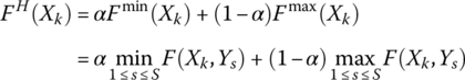
for a maximization problem or

for a minimization problem.
It allows one to construct q problems that, generally, include four or less (if not the all choice criteria are used in the analysis) objective functions as follows:
where ![]()
![]()
![]() and
and ![]()
Thus, the analysis of the solution alternatives and consequent choice of the rational solution alternatives can be realized within the framework of the <X, F> models. Applying Eqs. (4.31) or (4.32) to construct the corresponding membership functions for Fr, p(X), r = 1, 2, …, t, p = 1, 2, …, q, one can solve the problem Eq. (4.30) for the solution alternatives Xk, k = 1, 2, …, K. This method of analysis provides the choice of the rational solution alternatives in accordance with the principle of the Pareto optimality (Pareto 1886) and permits one to overcome the limitations of the generalization of the classic approach to dealing with the uncertainty of information indicated previously. Taking this into account, the payoff matrix with characteristic estimates (Table 6.2) is to be presented as the payoff matrix with the choice criteria estimates for p = 1, 2, …, q (Table 7.15) or for simplicity as the matrix of choice criteria estimates p = 1, 2, …, q (Table 7.16).
The availability of q matrices with choice criteria estimates allows one, applying Eqs. (4.31) or (4.32), to construct q modified matrices of choice criteria estimates, as shown in Table 7.17.
Finally, the presence of q modified matrices of choice criteria estimates permits one to construct the aggregated matrix of choice criteria estimates by applying Eq. (4.28), as shown in Table 7.18. This matrix includes the estimates calculated on the basis of Eq. (4.29) to provide the choice of the rational solution alternatives using Eq. (4.30).
Table 7.15 Payoff matrix with choice criteria estimates for the pth objective function.
| Y1 | ⋯ | Ys | ⋯ | YS | |||||
| X1 | Fp(X1, Y1) | ⋯ | Fp(X1, Ys) | ⋯ | Fp(X1, YS) | ||||
| ⋯ | ⋯ | ⋯ | ⋯ | ⋯ | ⋯ | ⋯ | ⋯ | ⋯ | ⋯ |
| Xk | Fp(Xk, Y1) | ⋯ | Fp(Xk, Ys) | ⋯ | Fp(Xk, YS) | ||||
| ⋯ | ⋯ | ⋯ | ⋯ | ⋯ | ⋯ | ⋯ | ⋯ | ⋯ | ⋯ |
| XK | Fp(XK, Y1) | ⋯ | Fp(XK, Ys) | ⋯ | Fp(XK, YS) | ||||
Table 7.16 Matrix of choice criteria estimates for the pth objective function.
| X1 | ||||
| ⋯ | ⋯ | ⋯ | ⋯ | ⋯ |
| Xk | ||||
| ⋯ | ⋯ | ⋯ | ⋯ | ⋯ |
| XK | ||||
Table 7.17 Modified matrix of choice criteria estimates for the pth objective function.
| X1 | ||||
| ⋯ | ⋯ | ⋯ | ⋯ | ⋯ |
| Xk | ||||
| ⋯ | ⋯ | ⋯ | ⋯ | ⋯ |
| XK |
Table 7.18 Aggregated payoff matrix of choice criteria estimates.
| X1 | ||||
| ⋯ | ⋯ | ⋯ | ⋯ | ⋯ |
| Xk | ||||
| ⋯ | ⋯ | ⋯ | ⋯ | ⋯ |
| XK | ||||
Table 7.19 Example 7.3: Modified matrix of estimates for the Laplace choice criterion for the first objective function.
| X1 | 0.67 |
| X2 | 1 |
| X3 | 0 |
| X4 | 0.83 |
Table 7.20 Example 7.3: Modified matrix of estimates for the Laplace choice criterion for the second objective function.
| X1 | 0.25 |
| X2 | 1 |
| X3 | 0.75 |
| X4 | 0 |
Table 7.21 Example 7.3: Aggregated matrix of choice criteria estimates.
| X1 | 0.25 |
| X2 | 1 |
| X3 | 0 |
| X4 | 0 |
Applying Eq. (6.16), we can form S representative combinations of initial data, states of nature, or scenarios, presented in Table 7.23.
Table 7.22 Example 7.4: Points of the LPτ‐sequences in Q6.
| s | t = 1 | t = 2 | t = 3 | t = 4 | t = 5 | t = 6 |
| 1 | 0.500 | 0.500 | 0.500 | 0.500 | 0.500 | 0.500 |
| 2 | 0.250 | 0.750 | 0.250 | 0.750 | 0.250 | 0.750 |
| 3 | 0.750 | 0.250 | 0.750 | 0.250 | 0.750 | 0.250 |
| 4 | 0.125 | 0.625 | 0.875 | 0.875 | 0.625 | 0.125 |
| 5 | 0.625 | 0.125 | 0.375 | 0.375 | 0.125 | 0.625 |
| 6 | 0.375 | 0.375 | 0.625 | 0.125 | 0.875 | 0.875 |
| 7 | 0.875 | 0.875 | 0.125 | 0.625 | 0.375 | 0.375 |
Table 7.23 Example 7.4: Representative combinations of initial data, states of nature, or scenarios Ys, s = 1, 2, …, S.
| s | t = 1 | t = 2 | t = 3 | t = 4 | t = 5 | t = 6 |
| 1 | 3.00 | 13.00 | 8.00 | 6.00 | 4.00 | 5.00 |
| 2 | 2.85 | 13.65 | 7.60 | 6.30 | 3.80 | 5.25 |
| 3 | 3.15 | 12.35 | 8.40 | 5.70 | 4.20 | 4.75 |
| 4 | 2.93 | 12.68 | 8.20 | 5.55 | 4.30 | 5.38 |
| 5 | 2.78 | 13.33 | 8.60 | 6.45 | 4.10 | 4.63 |
| 6 | 3.08 | 12.03 | 7.80 | 5.85 | 3.70 | 5.13 |
| 7 | 3.23 | 13.98 | 7.40 | 6.15 | 3.90 | 4.88 |
The coordinates of points given in Table 7.23 serve as a basis for constructing the following seven (in accordance with the representative combinations of initial data, states of nature, or scenarios) multiobjective problems:
which are subject to the same constraints in Eqs. (7.17)–(7.20).
The solutions to these problems, obtained with the use of the Bellman–Zadeh approach to decision‐making in a fuzzy environment for analyzing <X, F> models, are the following:
- s = 1:
 ,
,  ,
,  for Eqs. (7.21) and (7.22)
 - s = 2:
 ,
,  ,
,  for Eqs. (7.23) and (7.24)
 - s = 3:
 ,
,  ,
,  for Eqs. (7.25) and (7.26)
 - s = 4:
 ,
,  ,
,  for Eqs. (7.27) and (7.28)
 - s = 5:
 ,
,  ,
,  for Eqs. (7.29) and (7.30)
 - s = 6:
 ,
,  ,
,  for Eqs. (7.31) and (7.32)
 - s = 7:
 ,
,  ,
,  for Eqs. (7.33) and (7.34)
Therefore, we can form the following four solution alternatives for the problem Eqs. (7.15)–(7.20):
Table 7.24 Example 7.4: Payoff matrix for the first objective function.
| Y1 | Y2 | Y3 | Y4 | Y5 | Y6 | Y7 | |
| X1 | 250.00 | 249.20 | 250.80 | 249.43 | 259.83 | 239.03 | 252.03 |
| X2 | 243.75 | 249.01 | 246.49 | 245.87 | 255.58 | 236.17 | 253.77 |
| X3 | 242.75 | 244.26 | 241.24 | 240.60 | 249.76 | 231.45 | 249.60 |
| X4 | 247.10 | 249.50 | 244.70 | 244.52 | 253.89 | 235.14 | 255.27 |
Substituting these solutions into Eqs. (7.21), (7.23), (7.25), (7.27), (7.29), (7.31), and (7.33), we can construct the payoff matrix for the first objective function (Table 7.24). When substituting them into Eqs. (7.22), (7.24), (7.26), (7.28), (7.30), (7.32), and (7.34), we construct the payoff matrix for the second objective function (Table 7.26).
Let us consider the solution of the monocriteria problem Eq. (7.15) subject to the constraints in Eqs. (7.17)–(7.20), analyzing the payoff matrix given in Table 7.24 (Pereira Jr. et al. 2015). The corresponding matrix of the choice criteria estimates is presented in Table 7.25.
The analysis of Table 7.25 indicates that the use of the choice Wald criterion permits one to choose the solution alternative XW = {X3}. The use of the Laplace choice criterion allows one to find XL = {X3}. The application of the Savage choice criterion leads to XS = {X3}. Finally, the use of the Hurwicz choice criterion with α = 0.75 generates XH = {X3} as well. In such a manner, the solution alternative X3 is to be considered as the solution to the monocriteria problem Eq. (7.15) with the constraints in Eqs. (7.17)–(7.20) with a high degree of confidence.
Let us consider the solution of the monocriteria problem Eq. (7.16) subject to the constraints in Eqs. (7.17)–(7.20) by analyzing the payoff matrix given in Table 7.26. The corresponding matrix of choice criteria estimates is presented in Table 7.27.
Table 7.25 Example 7.4: Matrix of choice criteria estimates for the first objective function.
| FW(Xk) | FL(Xk) | FS(Xk) | FH(Xk) | |
| X1 | 259.83 | 250.05 | 10.07 | 254.63 |
| X2 | 255.58 | 247.81 | 5.82 | 250.73 |
| X3 | 249.76 | 242.81 | 0.00 | 245.18 |
| X4 | 255.27 | 247.16 | 5.24 | 250.24 |
| 249.76 | 242.81 | 0.00 | 245.18 | |
| 259.83 | 250.05 | 10.07 | 254.63 |
Table 7.26 Example 7.4: Payoff matrix for the second objective function.
| Y1 | Y2 | Y3 | Y4 | Y5 | Y6 | Y7 | |
| X1 | 148.00 | 151.80 | 144.20 | 152.87 | 146.87 | 146.07 | 146.47 |
| X2 | 148.45 | 151.67 | 145.23 | 151.58 | 149.62 | 145.33 | 147.48 |
| X3 | 149.45 | 152.72 | 146.18 | 151.75 | 151.44 | 146.05 | 148.75 |
| X4 | 148.58 | 151.47 | 145.69 | 150.83 | 150.96 | 144.82 | 147.89 |
Table 7.27 Example 7.4: Matrix of choice criteria estimates for the second objective function.
| FW(Xk) | FL(Xk) | FS(Xk) | FH(Xk) | |
| X1 | 152.87 | 148.04 | 2.04 | 150.70 |
| X2 | 151.67 | 148.48 | 2.75 | 150.06 |
| X3 | 152.72 | 149.48 | 4.57 | 151.05 |
| X4 | 151.47 | 148.61 | 4.09 | 149.81 |
| 151.47 | 148.04 | 2.04 | 149.81 | |
| 152.87 | 149.48 | 4.57 | 151.05 |
The analysis of Table 7.27 shows that XW = {X4}, XL = {X1}, XS = {X1}, and XH = {X4}. In such a manner, the alternatives X1 and X4 are to be considered as the solutions to the monocriteria problem Eq. (7.16) with the constraints in Eqs. (7.17)–(7.20). Formally, these alternatives cannot be distinguished on the basis of information defined by the payoff matrix in Table 7.26.
Let us return to the problem described by expressions Eqs. (7.15)–(7.20). The information in Table 7.25 permits one to construct the modified matrix of choice criteria estimates for the first objective function (Table 7.28). The modified matrix of choice criteria estimates for the second objective function (Table 7.29) has been obtained on the basis of information given in Table 7.27.
The modified matrices of choice criteria estimates presented in Tables 7.28 and 7.29 result in the construction of the aggregated payoff matrix presented in Table 7.30.
Thus, in this case, the use of the choice criteria of Wald, Laplace, and Hurwicz leads to the same solution alternative: XW = XL = XH = {X4}. At the same time, the Savage criterion leads to the solution XS = {X2}. (By the way, the application of the results of Ekel et al. 2008, 2011; Pedrycz et al. 2011, discussed in Section 7.1, lead to other solution alternatives: XW = XL = XH = {X4} and XS = {X3}; Pedrycz et al. 2011.)
Table 7.28 Example 7.4: Modified matrix of choice criteria estimates for the first objective function.
| X1 | 0 | 0 | 0 | 0 |
| X2 | 0.42 | 0.31 | 0.42 | 0.41 |
| X3 | 1 | 1 | 1 | 1 |
| X4 | 0.45 | 0.40 | 0.48 | 0.46 |
Table 7.29 Example 7.4: Modified matrix of choice criteria estimates for the second objective function.
| X1 | 0 | 1 | 1 | 0.28 |
| X2 | 0.86 | 0.69 | 0.72 | 0.80 |
| X3 | 0.11 | 0 | 0 | 0 |
| X4 | 1 | 0.60 | 0.19 | 1 |
Table 7.30 Example 7.4: Aggregated payoff matrix of choice criteria estimates.
| X1 | 0 | 0 | 0 | 0 |
| X2 | 0.42 | 0.31 | 0.42 | 0.41 |
| X3 | 0.11 | 0 | 0 | 0 |
| X4 | 0.45 | 0.40 | 0.19 | 0.46 |
Thus, the solution alternatives X2 and X4 are the result of the processing of available quantitative information. As indicated previously, if the solving capacity related to quantitative information processing does not permit one to obtain unique solutions, it is necessary to use, at the final decision stage, qualitative information based on knowledge, experience, and intuition of experts involved in the decision‐making process; in particular, within the framework of <X, R> models.
7.3 Construction of Objectives and Elaboration of Representative Combination of Initial Data, States of Nature, or Scenarios using Qualitative Information
As it was indicated previously, diverse classes of problems exist whose essence requires the consideration of the objectives formed on the basis of qualitative information at all stages of the decision‐making process. Taking this into account, the present section mainly reflects the results (Ramalho et al. 2019) that permit one to generate solutions, including robust solutions, to multiobjective decision‐making problems on the basis of direct using qualitative information within the framework of the possibilistic approach implemented with the application of the generalization of the classic approach to dealing with the uncertainty of information. The construction of the objective functions on the basis of qualitative information preserves the homogeneous formulation of the objectives, discussed in Chapter 4.
The approach discussed in the present section is associated with the following stages (Ramalho 2017; Ramalho et al. 2019):
- Elicitation of preferences;
- Representation of preferences within multiplicative preference relations;
- Definition of preference vectors on the basis of the analytic hierarchy process (AHP);
- Aggregation of preferences and generation of representative combination of initial data, states of nature, or scenarios.
This approach is based on applying and combining the results of Yager (1978); Saaty et al. (2003, 2007); Kokshenev et al. (2015); and Ekel et al. (2016). In particular, Yager (1978) uses the Bellman–Zadeh approach to decision‐making in a fuzzy environment (Bellman and Zadeh 1970) in conjunction with the AHP (Saaty 1980) for analyzing multiattribute problems that include objectives with unequal importance levels. The construction of a linear programming model, where either coefficients of an objective function or coefficients of constraints are estimated from the AHP, is proposed in Saaty et al. (2003). Some examples of applying the Saaty’s results (Saaty et al. 2003) to solve problems of allocating intangible resources through binary linear programming are given in Saaty et al. (2007). Finally, the results by Kokshenev et al. (2015) and Ekel et al. (2016) are directed at the use of the ordered weighted average (OWA) operator to regulate the level of intercriterion compensation or the degree of optimism or risk appetite inherent to the decision attitude (Damodaran 2008; Palomares et al. 2012; Kokshenev et al. 2015) in multiattribute decision‐making.
7.3.1 Elicitation of Preferences
The objective functions formed on the basis of qualitative information are to include elements reflecting the preferences of one or more involved experts, expressed by the corresponding preference structures or formats. In this chapter, we consider the application of the following preference formats, described in Chapter 5:
- ordering of the alternatives;
- additive reciprocal fuzzy preference relations;
- nonreciprocal fuzzy preference relations;
- fuzzy estimates;
- multiplicative preference relations.
Taking this into account, it should be noted that the nonreciprocal fuzzy preference relations and fuzzy estimates are equivalent to a certain extent. In particular, if two alternatives xk ∈ X and xl ∈ X have fuzzy estimates with the membership functions μ(xk) and μ(xl), then the quantity NR (xk, xl) is the degree of preference μ(xk)≽μ(xl), while the quantity NR (xl, xk) is the degree of preference μ(xl)≽μ(xk). Using the concept of a generalized preference relation, discussed in Chapter 5, as well as Eqs. (5.27) and (5.28), the quantities NR (xk, xl) and NR (xl, xk) can be evaluated, respectively, as the follows:
where μR(xk, xl) and μR(xl, xk) are the membership functions of the corresponding fuzzy preference relations that, respectively, reflect the essence of the preferences of xk over xl and of xl over xk (for instance, as indicated in Chapter 5, “more attractive,” “more flexible,” etc.).
When the indicator in terms of which alternatives xk and xl are evaluated can be measured on a numerical scale, and if the essence of preference behind relation R is coherent with the natural order (≤) along the axis of measured values of this indicator, then Eqs. (7.35) and (7.36), respectively, are reduced to
If the indicator has a maximization character, similar to Eqs. (5.29) and (5.30), the correlations Eqs. (7.37) and (7.38) are to be written for xk ≥ xl and xl ≥ xk, respectively. Thus, the availability of fuzzy estimates for all xk ∈ X is essential to realize an automatic construction of NR(xk, xl).
To continue the consideration of the stages indicated before, let us suppose (Ramalho 2017; Ramalho et al. 2019) that a group of experts E = {e1, e2, e3, e4} expresses their preferences relative to a set of alternatives X = {x1, x2, x3, x4} from the perspective of the criterion C (for example, “Innovation Level”).
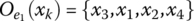
The expert e1 may express his/her preferences by the order of alternatives
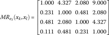
The expert e2 may express his/her preferences using the multiplicative preference relation, whose construction is based on Saaty (1980):

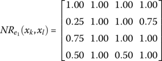
The expert e3 may present his/her preferences applying the fuzzy estimates shown in Figure 7.1 (these estimates have been borrowed from Queiroz 2009; however, it is possible to apply other types of fuzzy estimates), indicating the following: x1 – VH; x2 – VL; x3 – H; x4 – M. The use of Eqs. (7.37) and (7.38), modified for xk ≥ xl and xl ≥ xk, respectively, for these estimates permits one to construct the nonreciprocal fuzzy preference relation

Figure 7.1 Fuzzy set‐based qualitative scales utilized for objectives based on qualitative information.
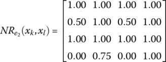
The expert e4 may also present his/her preferences applying the fuzzy estimates of Figure 7.1, indicating the following: x1 – H; x2 – M; x3 – M; x4 – L. It permits one, using Eqs. (7.33) and (7.34), also modified for xk ≥ xl and xl ≥ xk, to build

7.3.2 Representation of Preferences Within Multiplicative Preference Relations
As shown in Saaty et al. (2003), the components of the vector of preferences generated by the application of the AHP can be used as coefficients for forming the corresponding objective functions. The application of the AHP is based on processing the multiplicative preference relations. Thus, it is necessary to use transformation functions that permit one to convert different preference structures or formats (for example, ordering of alternatives, additive reciprocal fuzzy preference relations, and nonreciprocal fuzzy preference relations, etc.) to the multiplicative preference relations (Ramalho et al. 2019).
Taking this into account, it is necessary to indicate that there is not always a direct transformation of any preference format to the multiplicative preference relation. For instance, among preference formats discussed in Chapter 5, there is no direct conversion from the nonreciprocal fuzzy preference relations to the multiplicative fuzzy preference relations. It requires the preliminary conversion of the nonreciprocal fuzzy preference relations to the additive reciprocal fuzzy preference relations (Ramalho 2017; Ramalho et al. 2019).
Let us consider the transformation of the ordering of alternatives to the multiplicative preference relations. Applying the transformation function Eq. (5.40), we can obtain the additive reciprocal fuzzy preference relation from the ordering of alternatives. At the same time, the transformation function Eq. (5.50) permits one to generate the additive reciprocal fuzzy preference relation from the multiplicative preference relation. Substituting Eq. (5.50) in Eq. (5.40) and carrying out the corresponding transformations, one has
Accepting (as discussed in Chapter 5) the scale by Saaty (2008) with m = 9, it is possible to transform Eq. (7.43) as follows (Ramalho 2017; Ramalho et al. 2019):
Applying Eq. (7.44) to process Eq. (7.39), we can obtain

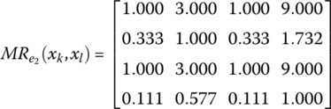
The application of the transformation function Eq. (5.53) permits one to obtain the following additive reciprocal fuzzy preference relations from Eqs. (7.41) and (7.42):

and

respectively.
The transformation function for constructing the multiplicative preference relations on the basis of the additive reciprocal fuzzy preference relations can be obtained from Eq. (5.51) and has the following form (Ramalho et al. 2019):
The use of Eq. (7.48) permits one to transform Eqs. (7.46) and (7.47) to

and

respectively.
7.3.3 Definition of Preference Vectors on the Basis of Applying the AHP
All the multiplicative preference relations in Eqs. have high levels of consistency: for all these multiplicative preference relations, the maximal eigenvalues λmax are close to the dimension n = 4 (Saaty 1980). Taking this into account, the eigenvectors corresponding to Eqs. (7.45), (7.40), (7.49), and (7.50), given as
and
can serve as the preference vectors.
The vectors in Eqs. (7.51)–(7.54) are to be aggregated and used as representative combinations of initial data, states of nature, or scenarios.
7.3.4 Aggregation of Preferences and Generation of Representative Combinations of Initial Data, States of Nature, or Scenarios
The central idea of this stage is to utilize the level of “orness”, offered by the OWA operator as a result of changing the set of the corresponding weights wi, i = 1, 2, …, n (as discussed in Chapter 4) and the generation of representative combinations of initial data, on the basis of applying the LPτ‐sequences, whose application was discussed in Chapter 6. This generation is to provide representative combinations of initial data, states of nature, or scenarios balanced from the point of view of a justified mixture of pessimistic and optimistic situations (Ramalho et al. 2019).
To implement this idea, it is first necessary to aggregate the opinions of the experts by extracting the limits of pessimism/optimism accepted by the DM. For instance, applying OWA ![]() for the vectors
for the vectors ![]() (pessimistic) and
(pessimistic) and ![]() (optimistic), respectively, it is possible (Ramalho et al. 2019) to obtain
(optimistic), respectively, it is possible (Ramalho et al. 2019) to obtain
and
The application of LPτ‐sequences is carried out taking into account the lower Eq. (7.55) and upper Eq. (7.56) limits for the generating, for example, S = 3 representative combinations of initial data, states of nature, or scenarios. It helps one to analyze the pth objective function with different coefficients
and
7.4 General Scheme of Multicriteria Decision‐Making under Conditions of Uncertainty
Taking into account the techniques presented previously, it is possible to suggest the general scheme of multicriteria decision‐making under conditions of information uncertainty, which is associated with the following stages:
- The first stage is related to constructing the objective functions. The procedure for building objective functions, based on quantitative indices and the direct application of LPτ‐sequences, is described Chapter 6. The objective functions formed on the basis of qualitative information are constructed with the application of results discussed in Section 7.3.
- The second stage consists in constructing q payoff matrices (in accordance with the number of objective functions considered) for all combinations of the given representative combination of initial data, solution alternatives, or scenarios Xk, k = 1, 2, …, K and the given representative states of nature Ys, s = 1, 2, …, S. To construct the payoff matrices, it is necessary to analyze S problems formalized within the framework of <X, F> models. The results of this analysis are the distinct solution alternatives Xk, k = 1, 2, …, K (K ≤ S). Thereafter, Xk, k = 1, 2, …, K are substituted into Fp(X), p = 1, 2, …, q for Ys, s = 1, 2, …, S. These substitutions generate q payoff matrices.
- The third stage is related to the analysis of the obtained payoff matrices. Its execution is based on the results presented in Sections 7.1 and 7.2. However, the insufficient resolving capacity of the present stage may lead to non‐unique solutions and the necessity of applying the fourth stage.
- The fourth stage is associated with constructing and analyzing <X, R> models for the subsequent contraction of decision uncertainty regions. In this stage, the remaining rational solutions should be analyzed by applying additional criteria, including criteria based on knowledge, experience, and intuition of involved experts.
The flow chart in Figure 7.2 illustrates the general scheme described previously. This scheme can be used to construct solutions, including robust solutions, in multiobjective analysis under conditions of uncertainty (Ramalho 2017; Ramalho et al. 2019).
Figure 7.2 Flow chart of the general scheme of multiobjective decision‐making under information uncertainty.
7.5 Application Studies
As examples illustrating the results of the present chapter, we consider the problems of multiobjective allocation of a shortage of financial resources in strategic planning formed on the basis of quantitative information as well as of quantitative and qualitative information (Ramalho et al. 2019). These problems are resolved within model 3 of allocating resources or their shortages, discussed in Section 4.7.
Thus, we have to consider the following constraint:
Besides, we have to take into account that
and
Table 7.31 Example 7.5: Initial information for shortage allocation.
| Project | Di, kU$ | Ai, kU$ | |
| 1 | 12 532.00 | 10 020.00 | 2512.00 |
| 2 | 17 528.00 | 16 130.00 | 1398.00 |
| 3 | 9744.00 | 7768.00 | 1976.00 |
| 4 | 19 123.00 | 16 230.00 | 2910.00 |
The objectives are the following:
- Prevailing financial constraint of projects generating a lower level of product supply abroad;
- Prevailing financial constraint of projects generating a lower level of profit for each invested U$ 1 000 000.00.
The initial information needed for constructing objective functions corresponding to these objectives is presented in Table 7.32.
The application of LPτ‐sequences, considering the lower and upper limits given in Table 7.32 for generating, for example, S = 7 representative combinations of initial data, states of nature, or scenarios, gives rise to the following seven multiobjective problems:
Table 7.32 Example 7.5: Initial information for constructing objective functions.
| Project | ||
| 1 | [20.50, 31.50] | [2210.00, 2850.00] |
| 2 | [42.50, 49.50] | [1850.00, 2350.00] |
| 3 | [25.50, 33.50] | [1700.00, 1950.00] |
| 4 | [10.50, 14.50] | [2340.00, 2950.00] |
which are subject to the same constraints in Eqs. (7.61)–(7.64).
Using the results, discussed in Chapter 4, for analyzing these problems one can obtain the solutions given in Table 7.33. Substituting these solutions into Eqs. (7.65), (7.67), (7.69), (7.71), (7.73), (7.75), and (7.77), we can construct the payoff matrix for the first objective function (Table 7.34). Substituting these solutions into Eqs. (7.66), (7.68), (7.70), (7.72), (7.74), (7.76), and (7.78), we can construct the payoff matrix for the second objective function (Table 7.35).
The results presented in Tables 7.34 and 7.35 allow us to construct the characteristic estimates given in Tables 7.36 and 7.37. Then, we can apply Eqs. (7.9)–(7.11) and (7.13) to construct the matrices with the choice criteria estimates shown in Tables 7.38 and 7.39.
Applying Eq. (4.31) to the choice criteria estimates, we construct the corresponding modified matrices presented in Tables 7.40 and 7.41. The application of Eq. (4.28) to the modified matrices with the choice criteria estimates results in the construction of the matrix with the aggregated levels of the fuzzy choice criteria given in Table 7.42.
Table 7.33 Example 7.5: Solution alternatives for S = 7 scenarios.
| Solution | Δx1 | Δx2 | Δx3 | Δx4 |
| 1 | 1981.214 | 642.887 | 1976.000 | 2626.899 |
| 2 | 1971.689 | 360.733 | 1976.000 | 2618.578 |
| 3 | 2083.692 | 340.168 | 1976.000 | 2527.139 |
| 4 | 2221.119 | 69.114 | 1976.000 | 2660.768 |
| 5 | 2244.887 | 185.166 | 1976.000 | 2520.947 |
| 6 | 2440.874 | 59.381 | 1976.000 | 2450.745 |
| 7 | 2512.000 | 183.686 | 1976.000 | 2255.314 |
Table 7.34 Example 7.5: Payoff matrix for the first objective function.
| Solution | Y1 | Y2 | Y3 | Y4 | Y5 | Y6 | Y7 |
| ΔX1 | 164 412.62 | 159 589.23 | 169 236.00 | 167 908.48 | 161 747.26 | 159 574.07 | 168 420.65 |
| ΔX2 | 158 881.86 | 152 757.58 | 165 006.14 | 160 920.15 | 157 360.72 | 153 903.28 | 163 343.29 |
| ΔX3 | 159 704.99 | 153 145.27 | 166 264.71 | 161 126.11 | 158 437.55 | 154 727.55 | 164 528.73 |
| ΔX4 | 152 479.92 | 145 201.56 | 159 758.28 | 153 297.43 | 152 046.15 | 147 350.25 | 157 225.84 |
| ΔX5 | 156 688.54 | 149 408.09 | 163 968.99 | 157 299.82 | 156 052.73 | 151 634.38 | 161 767.24 |
| ΔX6 | 155 120.56 | 147 010.82 | 163 230.30 | 154 708.03 | 155 119.52 | 150 012.29 | 160 642.42 |
| ΔX7 | 160 244.97 | 151 961.74 | 168 528.21 | 159 354.67 | 160 113.14 | 155 223.28 | 166 288.81 |
Table 7.35 Example 7.5: Payoff matrix for the second objective function.
| Solution | Y1 | Y2 | Y3 | Y4 | Y5 | Y6 | Y7 |
| ΔX1 | 16 157 881.78 | 16 246 350.54 | 16 069 413.02 | 15 909 786.48 | 16 580 723.10 | 16 696 965.53 | 15 444 051.12 |
| ΔX2 | 16 278 251.23 | 16 283 705.90 | 16 272 796.56 | 16 106 932.25 | 16 611 841.59 | 16 833 510.54 | 15 560 720.54 |
| ΔX3 | 16 276 578.63 | 16 247 597.69 | 16 305 559.57 | 16 125 048.06 | 16 561 086.18 | 16 847 890.71 | 15 572 289.59 |
| ΔX4 | 16 408 499.27 | 16 344 026.60 | 16 472 971.94 | 16 308 596.36 | 16 673 651.02 | 16 972 160.10 | 15 679 589.59 |
| ΔX5 | 16 342 517.42 | 16 267 425.69 | 16 417 609.16 | 16 233 417.51 | 16 577 234.04 | 16 922 981.15 | 15 636 436.98 |
| ΔX6 | 16 388 531.83 | 16 255 653.26 | 16 521 410.40 | 16 324 048.48 | 16 552 291.34 | 16 987 094.82 | 15 690 692.67 |
| ΔX7 | 16 312 606.25 | 16 154 082.39 | 16 471 130.11 | 16 245 407.46 | 16 422 359.74 | 16 936 645.04 | 15 646 012.76 |
Table 7.36 Example 7.5: Matrix with the characteristic estimates for the first objective function.
| Solution | Fmax(ΔXk) | Fmin(ΔXk) | rmax(ΔXk) | |
| ΔX1 | 164 412.62 | 159 589.23 | 169 236.00 | 167 908.48 |
| ΔX2 | 158 881.86 | 152 757.58 | 165 006.14 | 160 920.15 |
| ΔX3 | 159 704.99 | 153 145.27 | 166 264.71 | 161 126.11 |
| ΔX4 | 152 479.92 | 145 201.56 | 159 758.28 | 153 297.43 |
| ΔX5 | 156 688.54 | 149 408.09 | 163 968.99 | 157 299.82 |
| ΔX6 | 155 120.56 | 147 010.82 | 163 230.30 | 154 708.03 |
| ΔX7 | 160 244.97 | 151 961.74 | 168 528.21 | 159 354.67 |
Table 7.37 Example 7.5: Matrix with the characteristic estimates for the second objective function.
| Solution | Fmax(ΔXk) | Fmin(ΔXk) | rmax(ΔXk) | |
| ΔX1 | 16 696 965.53 | 15 444 051.12 | 16 157 881.78 | 158 364.26 |
| ΔX2 | 16 833 510.54 | 15 560 720.54 | 16 278 251.23 | 203 383.53 |
| ΔX3 | 16 847 890.71 | 15 572 289.59 | 16 276 578.63 | 236 146.55 |
| ΔX4 | 16 972 160.10 | 15 679 589.59 | 16 408 499.27 | 403 558.91 |
| ΔX5 | 16 922 981.15 | 15 636 436.98 | 16 342 517.42 | 348 196.13 |
| ΔX6 | 16 987 094.82 | 15 690 692.67 | 16 388 531.83 | 451 997.38 |
| ΔX7 | 16 936 645.04 | 15 646 012.76 | 16 312 606.25 | 401 717.09 |
Table 7.38 Example 7.5: Matrix with the choice criteria estimates for the first objective function.
| Solution | ||||
| ΔX1 | 169 236.00 | 164 412.62 | 14 611.05 | 161 989.55 |
| ΔX2 | 165 006.14 | 158 881.86 | 7622.72 | 155 819.72 |
| ΔX3 | 166 264.70 | 159 704.99 | 7943.71 | 156 425.13 |
| ΔX4 | 159 758.28 | 152 479.92 | 0.000 | 148 840.74 |
| ΔX5 | 163 968.99 | 156 688.54 | 4541.40 | 153 048.32 |
| ΔX6 | 163 230.30 | 155 120.56 | 3472.03 | 151 065.69 |
| ΔX7 | 168 528.21 | 160 244.97 | 9062.97 | 156 103.36 |
| 159 758.28 | 152 479.92 | 0.000 | 148 840.74 | |
| 169 236.00 | 164 412.62 | 14 611.05 | 161 989.55 |
Table 7.39 Example 7.5: Matrix with the choice criteria estimates for the second objective.
| Solution | ||||
| ΔX1 | 16 696 965.53 | 16 157 881.78 | 158 364.26 | 15 757 279.76 |
| ΔX2 | 16 833 510.54 | 16 278 251.23 | 203 383.53 | 15 878 918.04 |
| ΔX3 | 16 847 890.71 | 16 276 578.63 | 236 146.55 | 15 891 189.87 |
| ΔX4 | 16 972 160.10 | 16 408 499.27 | 403 558.91 | 16 002 732.25 |
| ΔX5 | 16 922 981.15 | 16 342 517.42 | 348 196.13 | 15 958 073.02 |
| ΔX6 | 16 987 094.82 | 16 388 531.83 | 451 997.38 | 16 014 793.24 |
| ΔX7 | 16 936 645.04 | 16 312 606.25 | 401 717.09 | 15 968 670.83 |
| 16 696 965.53 | 16 157 881.78 | 158 364.26 | 15 757 279.76 | |
| 16 987 094.82 | 16 408 499.27 | 451 997.38 | 16 014 793.21 |
Table 7.40 Example 7.5: Modified matrix with the choice criteria estimates for the first objective function.
| ΔX1 | 0.00 | 0.00 | 0.00 | 0.00 |
| ΔX2 | 0.45 | 0.46 | 0.48 | 0.47 |
| ΔX3 | 0.31 | 0.40 | 0.46 | 0.42 |
| ΔX4 | 1.00 | 1.00 | 1.00 | 1.00 |
| ΔX5 | 0.56 | 0.65 | 0.69 | 0.68 |
| ΔX6 | 0.63 | 0.78 | 0.76 | 0.83 |
| ΔX7 | 0.08 | 0.35 | 0.38 | 0.45 |
Table 7.41 Example 7.5: Modified matrix with the choice criteria estimates for the second objective function.
| Solution | ||||
| ΔX1 | 1.00 | 1.00 | 1.00 | 1.00 |
| ΔX2 | 0.53 | 0.52 | 0.85 | 0.53 |
| ΔX3 | 0.48 | 0.53 | 0.74 | 0.48 |
| ΔX4 | 0.05 | 0.00 | 0.17 | 0.05 |
| ΔX5 | 0.22 | 0.26 | 0.35 | 0.22 |
| ΔX6 | 0.00 | 0.08 | 0.00 | 0.00 |
| ΔX7 | 0.17 | 0.38 | 0.17 | 0.18 |
Table 7.42 Example 7.5: Matrix with the aggregated levels of the fuzzy choice criteria.
| ΔX1 | 0.00 | 0.00 | 0.00 | 0.00 |
| ΔX2 | 0.45 | 0.46 | 0.48 | 0.47 |
| ΔX3 | 0.31 | 0.40 | 0.46 | 0.42 |
| ΔX4 | 0.05 | 0.00 | 0.17 | 0.05 |
| ΔX5 | 0.22 | 0.26 | 0.35 | 0.22 |
| ΔX6 | 0.00 | 0.08 | 0.00 | 0.00 |
| ΔX7 | 0.08 | 0.35 | 0.17 | 0.18 |
| 0.45 | 0.46 | 0.48 | 0.47 |
The results presented in Table 7.42 convincingly demonstrate that problem solution is ![]() . However, if the aggregated fuzzy choice criteria levels indicate different solutions (the quantitative information does not lead to a unique solution), it is possible to apply the criteria of qualitative character at the final decision stage.
. However, if the aggregated fuzzy choice criteria levels indicate different solutions (the quantitative information does not lead to a unique solution), it is possible to apply the criteria of qualitative character at the final decision stage.
The objectives are the following:
- Prevailing financial constraint of projects generating a lower level of product supply abroad.
- Prevailing financial constraint of projects generating a lower level of profit for each invested U$ 1 000 000.00.
- Prevailing financial constraint of projects generating a lower level of innovation.
The constraints of the modified problem are the same as the previous problem, defined in Eqs. (7.61)–(7.64). The first two objective functions are the same as in the previous example. The construction of the third objective function is based on the use of qualitative information. This information is provided by a group of experts E = {e1, e2, e3}, responsible for generating the necessary estimates related to a set of projects X = {x1, x2, x3, x4} from the perspective of the indicator “Level of Innovation.”
In particular, the expert e1 has presented his/her preferences applying the fuzzy estimates of Figure 7.1, indicating the following: x1 − VH; x2 − L; x3 − H; x4 − M. The expert e2 has also used the fuzzy estimates of Figure 7.1 and indicated x1 − H; x2 − M; x3 − H; x4 − L. Finally, the expert e3 has ordered the alternatives as follows:
The first step in the problem solution is the processing of qualitative information for the construction of estimates for the third objective function. From the fuzzy estimates given by the experts e1 and e2, on the basis of Figure 7.1, and applying Eqs. (7.37) and (7.38), one can obtain the following nonreciprocal fuzzy preference relations:
and
Then, by applying Eq. (5.48), Eqs. (7.80) and (7.81) are converted into the reciprocal fuzzy preference relations

and

respectively.
Applying Eqs. (7.48) to Eqs. (7.82) and (7.83), we construct the multiplicative preference relations

and
respectively.
As the expert e3 has expressed his/her preferences by Eq. (7.79), applying Eq. (7.44) to Eq. (7.79), we construct the following multiplicative preference relation:
All the multiplicative preference relations Eqs. (7.84)–(7.86) have high levels of consistency: for all of them the maximal eigenvalues λmax are close to the dimensionality of the relations (n = 4). Considering this, the eigenvectors corresponding to Eqs. (7.84)–(7.86)
and
can serve as vectors of preferences.
On the basis of Eqs. (7.87)–(7.89) one can construct
and
Considering the lower Eq. (7.90) and upper Eq. (7.91) limits for the objective, based on the use of qualitative information, and the other two objectives, based on the application of quantitative information, we can now resume the second stage of the general scheme of multicriteria decision‐making under conditions of information uncertainty. Therefore, we can use the LPτ‐sequences for generating, for example, S = 7 representative combinations of initial data, states of nature, or scenarios. It gives rise to the following seven multiobjective problems:
which are subject to the constraints in Eqs. (7.61)–(7.64).
Using the Bellman–Zadeh approach presented in Chapter 4 for analyzing the problems in Eqs. (7.92)–(7.112), one can construct Table 7.43. Substituting these solutions into Eqs. (7.92), (7.95), (7.98), (7.101), (7.104), (7.107), and (7.110), we construct the payoff matrix for the first objective function (Table 7.44). Substituting these solutions into Eqs. (7.93), (7.9), (7.99), (7.102), (7.105), (7.108), and (7.111), the payoff matrix for the second objective function is constructed (Table 7.45). Finally, substituting the same solutions into Eqs (7.94), (7.97), (7.100), (7.103), (7.106), (7.109), and (7.112), we construct the payoff matrix for the third objective function (Table 7.46).
The results shown in Tables 7.44–7.46 produce matrices with the characteristic estimates presented in Tables 7.47–7.49 and the corresponding matrices with the choice criteria estimates are given in Tables 7.50–7.52. Applying Eq. (4.31) to these estimates, we construct the corresponding modified matrices, presented in Tables 7.53–7.55. The modified matrices with the choice criteria estimates result in the construction of the matrix with the aggregated levels of the fuzzy choice criteria, presented in Table 7.56.
Finally, the problem’s solution is ![]() ,
, ![]() ,
, ![]() ,
, ![]() , which differs significantly from the solution obtained with considering only the objective functions formed on the basis of quantitative information, presented in Example 7.5. Once we found a single solution to the problem, there is no need to apply the fourth stage of the general scheme of multicriteria decision‐making under conditions of information uncertainty.
, which differs significantly from the solution obtained with considering only the objective functions formed on the basis of quantitative information, presented in Example 7.5. Once we found a single solution to the problem, there is no need to apply the fourth stage of the general scheme of multicriteria decision‐making under conditions of information uncertainty.
Table 7.43 Example 7.6: Solution alternatives for S = 7 scenarios.
| Solution | Δx1 | Δx2 | Δx3 | Δx4 |
| 1 | 1183.09 | 1398.00 | 1435.91 | 2910.00 |
| 2 | 1193.59 | 858.84 | 1976.00 | 2898.58 |
| 3 | 1294.36 | 947.73 | 1830.68 | 2854.24 |
| 4 | 1390.00 | 1329.14 | 1297.86 | 2901.00 |
| 5 | 1560.76 | 888.64 | 1589.21 | 2888.39 |
| 6 | 1569.50 | 797.19 | 1716.70 | 2843.62 |
| 7 | 2272.74 | 304.83 | 1439.44 | 2910.00 |
Table 7.44 Example 7.6: Payoff matrix for the first objective function.
| Solution | Y1 | Y2 | Y3 | Y4 | Y5 | Y6 | Y7 |
| ΔX1 | 173 802.68 | 173 033.86 | 174 571.50 | 178 818.39 | 168 868.78 | 168 023.58 | 179 499.97 |
| ΔX2 | 165 063.94 | 162 231.11 | 167 896.77 | 171 167.73 | 161 025.39 | 160 299.41 | 167 763.22 |
| ΔX3 | 166 931.72 | 164 223.62 | 169 639.81 | 172 195.13 | 162 965.89 | 161 872.04 | 170 693.82 |
| ΔX4 | 171 942.32 | 170 760.10 | 173 124.55 | 175 630.15 | 167 611.72 | 165 800.94 | 178 726.48 |
| ΔX5 | 164 443.82 | 161 416.82 | 167 470.83 | 167 883.47 | 161 223.78 | 158 776.85 | 169 891.19 |
| ΔX6 | 163 665.30 | 160 154.50 | 167 176.11 | 167 304.19 | 160 592.23 | 158 260.97 | 168 503.79 |
| ΔX7 | 151 951.54 | 146 266.09 | 157 637.00 | 151 526.53 | 151 381.96 | 145 634.24 | 159 263.45 |
Table 7.45 Example 7.6: Payoff matrix for the second objective function.
| Solution | Y1 | Y2 | Y3 | Y4 | Y5 | Y6 | Y7 |
| ΔX1 | 16 246 505.72 | 16 585 991.54 | 15 907 019.91 | 15 812 268.65 | 16 850 216.95 | 16 879 844.40 | 15 443 692.89 |
| ΔX2 | 16 096 266.88 | 16 331 180.09 | 15 861 353.66 | 15 747 955.80 | 16 711 782.23 | 16 579 526.17 | 15 345 803.31 |
| ΔX3 | 16 155 396.78 | 16 387 618.28 | 15 923 175.29 | 15 806 402.91 | 16 728 515.46 | 16 689 751.31 | 15 396 917.45 |
| ΔX4 | 16 373 437.98 | 16 679 839.11 | 16 067 036.85 | 15 972 978.62 | 16 910 246.03 | 17 056 464.75 | 15 554 062.52 |
| ΔX5 | 16 354 964.30 | 16 557 476.42 | 16 152 452.18 | 16 043 302.35 | 16 845 629.68 | 16 967 417.49 | 15 563 507.68 |
| ΔX6 | 16 299 263.71 | 16 474 150.88 | 16 124 376.55 | 16 004 878.25 | 16 783 827.30 | 16 881 300.51 | 15 527 048.80 |
| ΔX7 | 16 714 082.22 | 16 742 357.56 | 16 685 806.89 | 16 571 876.55 | 16 988 286.35 | 17 403 634.48 | 15 892 531.50 |
Table 7.46 Example 7.6: Payoff matrix for the third objective function.
| Solution | Y1 | Y2 | Y3 | Y4 | Y5 | Y6 | Y7 |
| ΔX1 | 1442.49 | 1463.72 | 1421.25 | 1615.90 | 1283.59 | 1414.00 | 1456.47 |
| ΔX2 | 1578.05 | 1628.57 | 1527.53 | 1757.48 | 1401.73 | 1525.97 | 1627.01 |
| ΔX3 | 1581.89 | 1629.75 | 1534.02 | 1763.29 | 1410.25 | 1529.13 | 1624.87 |
| ΔX4 | 1488.72 | 1512.92 | 1464.52 | 1669.54 | 1335.68 | 1450.63 | 1499.03 |
| ΔX5 | 1625.65 | 1673.90 | 1577.40 | 1816.53 | 1464.12 | 1562.73 | 1659.23 |
| ΔX6 | 1660.37 | 1715.90 | 1604.84 | 1852.18 | 1494.13 | 1592.06 | 1703.12 |
| ΔX7 | 1863.73 | 1939.47 | 1787.99 | 2083.95 | 1712.26 | 1753.61 | 1905.10 |
Table 7.47 Example 7.6: Matrix with the characteristic estimates for the first objective function.
| Solution | Fmax(ΔXk) | Fmin(ΔXk) | rmax(ΔXk) | |
| ΔX1 | 179 499.97 | 168 023.58 | 173 802.68 | 27 291.86 |
| ΔX2 | 171 167.73 | 160 299.41 | 165 063.94 | 19 641.20 |
| ΔX3 | 172 195.13 | 161 872.04 | 166 931.72 | 20 668.59 |
| ΔX4 | 178 726.48 | 165 800.94 | 171 942.32 | 24 494.01 |
| ΔX5 | 169 891.19 | 158 776.85 | 164 443.82 | 16 356.94 |
| ΔX6 | 168 503.79 | 158 260.97 | 163 665.30 | 15 777.66 |
| ΔX7 | 159 263.45 | 145 634.24 | 151 951.54 | 0.00 |
Table 7.48 Example 7.6: Matrix with the characteristic estimates for the second objective function.
| Solution | Fmax(ΔXk) | Fmin(ΔXk) | rmax(ΔXk) | |
| ΔX1 | 16 879 844.40 | 15 443 692.89 | 16 246 505.72 | 300 318.24 |
| ΔX2 | 16 711 782.23 | 15 345 803.31 | 16 096 266.88 | 0.00 |
| ΔX3 | 16 728 515.46 | 15 396 917.45 | 16 155 396.78 | 110 225.14 |
| ΔX4 | 17 056 464.75 | 15 554 062.52 | 16 373 437.98 | 476 938.59 |
| ΔX5 | 16 967 417.49 | 15 563 507.68 | 16 354 964.30 | 387 891.32 |
| ΔX6 | 16 881 300.51 | 15 527 048.80 | 16 299 263.71 | 301 774.34 |
| ΔX7 | 17 403 634.48 | 15 892 531.50 | 16 714 082.22 | 824 453.22 |
Table 7.49 Example 7.6: Matrix with the characteristic estimates for the third objective.
| Solution | Fmax(ΔXk) | Fmin(ΔXk) | rmax(ΔXk) | |
| ΔX1 | 1615.899 | 1283.586 | 1442.487 | 0.000 |
| ΔX2 | 1757.480 | 1401.731 | 1578.050 | 170.548 |
| ΔX3 | 1763.294 | 1410.247 | 1581.885 | 168.402 |
| ΔX4 | 1669.536 | 1335.676 | 1488.718 | 53.637 |
| ΔX5 | 1816.528 | 1464.123 | 1625.653 | 210.182 |
| ΔX6 | 1852.183 | 1494.132 | 1660.373 | 252.181 |
| ΔX7 | 2083.953 | 1712.262 | 1863.730 | 475.750 |
Table 7.50 Example 7.6: Matrix with the choice criteria estimates for the first objective function.
| ΔX1 | 179 499.97 | 173 802.68 | 27 291.86 | 170 892.68 |
| ΔX2 | 171 167.73 | 165 063.94 | 19 641.20 | 163 016.49 |
| ΔX3 | 172 195.13 | 166 931.72 | 20 668.59 | 164 452.81 |
| ΔX4 | 178 726.48 | 171 942.32 | 24 494.01 | 169 032.32 |
| ΔX5 | 169 891.19 | 164 443.82 | 16 356.94 | 161 555.44 |
| ΔX6 | 168 503.79 | 163 665.30 | 15 777.66 | 160 821.68 |
| ΔX7 | 159 263.45 | 151 951.54 | 0.00 | 149 041.55 |
| 159 263.45 | 151 951.54 | 0.00 | 149 041.55 | |
| 179 499.97 | 173 802.68 | 27 291.86 | 170 892.68 |
Table 7.51 Example 7.6: Matrix with the choice criteria estimates for the second objective function.
| ΔX1 | 16 879 844.40 | 16 246 505.72 | 300 318.24 | 15 802 730.77 |
| ΔX2 | 16 711 782.23 | 16 096 266.88 | 0.00 | 15 687 298.04 |
| ΔX3 | 16 728 515.46 | 16 155 396.78 | 110 225.14 | 15 729 816.95 |
| ΔX4 | 17 056 464.75 | 16 373 437.98 | 476 938.59 | 15 929 663.07 |
| ΔX5 | 16 967 417.49 | 16 354 964.30 | 387 891.32 | 15 914 485.13 |
| ΔX6 | 16 881 300.51 | 16 299 263.71 | 301 774.34 | 15 865 611.73 |
| ΔX7 | 17 403 634.48 | 16 714 082.22 | 824 453.22 | 16 270 307.24 |
| 16 711 782.23 | 16 096 266.88 | 0.00 | 15 687 298.04 | |
| 17 403 634.48 | 16 714 082.22 | 824 453.22 | 16 270 307.24 |
Table 7.52 Example 7.6: Matrix with the choice criteria estimates for the third objective function.
| ΔX1 | 1615.90 | 1442.49 | 0.00 | 1366.66 |
| ΔX2 | 1757.48 | 1578.05 | 170.55 | 1490.67 |
| ΔX3 | 1763.29 | 1581.89 | 168.40 | 1498.51 |
| ΔX4 | 1669.54 | 1488.72 | 53.64 | 1419.14 |
| ΔX5 | 1816.53 | 1625.65 | 210.18 | 1552.22 |
| ΔX6 | 1852.18 | 1660.37 | 252.18 | 1583.65 |
| ΔX7 | 2083.95 | 1863.73 | 475.75 | 1805.19 |
| 1615.90 | 1442.49 | 0.00 | 1366.66 | |
| 2083.95 | 1863.73 | 475.75 | 1805.19 |
Table 7.53 Example 7.6: Modified matrix with the choice criteria estimates for the first objective function.
| ΔX1 | 0.00 | 0.00 | 0.00 | 0.00 |
| ΔX2 | 0.41 | 0.40 | 0.28 | 0.36 |
| ΔX3 | 0.36 | 0.31 | 0.24 | 0.30 |
| ΔX4 | 0.04 | 0.09 | 0.10 | 0.09 |
| ΔX5 | 0.48 | 0.43 | 0.40 | 0.43 |
| ΔX6 | 0.54 | 0.46 | 0.42 | 0.46 |
| ΔX7 | 1.00 | 1.00 | 1.00 | 1.00 |
Table 7.54 Example 7.6: Modified matrix with the choice criteria estimates for the second objective function.
| ΔX1 | 0.76 | 0.76 | 0.64 | 0.80 |
| ΔX2 | 1.00 | 1.00 | 1.00 | 1.00 |
| ΔX3 | 0.98 | 0.90 | 0.87 | 0.93 |
| ΔX4 | 0.50 | 0.55 | 0.42 | 0.58 |
| ΔX5 | 0.63 | 0.58 | 0.53 | 0.61 |
| ΔX6 | 0.76 | 0.67 | 0.63 | 0.69 |
| ΔX7 | 0.00 | 0.00 | 0.00 | 0.00 |
Table 7.55 Example 7.6: Modified matrix with the choice criteria estimates for the third objective function.
| ΔX1 | 1.00 | 1.00 | 1.00 | 1.00 |
| ΔX2 | 0.70 | 0.68 | 0.64 | 0.72 |
| ΔX3 | 0.69 | 0.67 | 0.65 | 0.70 |
| ΔX4 | 0.89 | 0.89 | 0.89 | 0.88 |
| ΔX5 | 0.57 | 0.57 | 0.56 | 0.58 |
| ΔX6 | 0.50 | 0.48 | 0.47 | 0.51 |
| ΔX7 | 0.00 | 0.00 | 0.00 | 0.00 |
Table 7.56 Example 7.6: Aggregated payoff matrix of choice criteria estimates.
| ΔX1 | 0.00 | 0.00 | 0.00 | 0.00 |
| ΔX2 | 0.41 | 0.40 | 0.28 | 0.36 |
| ΔX3 | 0.36 | 0.31 | 0.24 | 0.30 |
| ΔX4 | 0.04 | 0.09 | 0.10 | 0.09 |
| ΔX5 | 0.48 | 0.43 | 0.40 | 0.43 |
| ΔX6 | 0.50 | 0.46 | 0.42 | 0.46 |
| ΔX7 | 0.00 | 0.00 | 0.00 | 0.00 |
| maxμD(Xk) | 0.50 | 0.46 | 0.42 | 0.46 |
7.6 Conclusions
We have considered the use of the choice criteria of the classic approach to handle information uncertainty in monocriteria decision‐making as objective functions within the framework of multiobjective models. This consideration has permitted us to propose the general methodology for multicriteria decision‐making under conditions of uncertainty. The proposed methodology is based on a possibilistic approach to produce solutions, including robust solutions, in multicriteria analysis. Its use allows one to use available quantitative information to the highest degree to reduce the decision uncertainty regions. If the solving capacity of quantitative information processing does not permit one to obtain unique solutions, the methodology supposes the utilization, at the final decision stage, of qualitative information within the framework of <X, R > models. Thus, the general scheme is based on combining <X, F > models, <X, R > models, and the generalization of the classic approach to dealing with uncertainty of information.
However, in recent years, problems have appeared more often that require the consideration of the objectives formed with the use of qualitative information, at all stages, from the beginning of the decision‐making process. Considering this, in this chapter an approach has been described that permits one to generate robust multiobjective solutions (within the framework of the possibilistic approach) by constructing representative combinations of initial data, states of nature, or scenarios with the direct use of qualitative information along with quantitative information, assuring convincing information fusion. The approach admits the possibility for experts to apply diverse preference formats with their processing on the basis of different transformation functions.
Exercises
- 7.1 Apply the approach described in Section 7.1, associated with constructing an aggregated payoff matrix, to analyze a bicriteria decision‐making problem related to considering the solution alternatives Xk, k = 1, 2, …, 4 with the presence of the representative combinations of initial data, states of nature, or scenarios Ys, s = 1, 2, …, 4. Both objective functions are to be minimized. The corresponding payoff matrices are presented in Tables 7.57 and 7.58. Also, take into consideration α = 0.75 in applying the Hurwicz choice criterion.
Table 7.57 Problem 7.1: Payoff matrix for the first criterion.
Y1 Y2 Y3 Y4 X1 2 3 3 5 X2 7 1 2 3 X3 3 8 2 6 X4 1 5 8 4 Table 7.58 Problem 7.1: Payoff matrix for the second criterion.
Y1 Y2 Y3 Y4 X1 9 3 4 8 X2 8 5 3 8 X3 6 6 9 4 X4 7 2 4 7 - 7.2 Solve the problem given in Problem 7.1 by applying the approach to dealing with uncertainty of information based on considering the choice criteria as objective functions, discussed in Section 7.2.
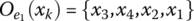
- 7.3 Suppose that members of a group of experts E = {e1, e2, e3} presented their preferences relatively to a set of alternatives X = {x1, x2, x3, x4}. The expert e1 expressed his/her preferences by the order of alternatives
 . The experts e2 and e3 presented their preferences applying the fuzzy estimates shown in Figure 7.1, indicating the following: x1 – H; x2 – L; x3 – M; x4 – VH and x1 – M; x2 – H; x3 – VH; x4 – M, respectively. Based on the preferences given here, construct the corresponding multiplicative preference relations for each expert.
 - 7.4 Based on the multiplicative preference relations, obtained in solving Problem 7.3, find the eigenvectors to define the preference vectors for each expert. Then, applying OWA
 for the vectors
  (pessimistic) and
  (optimistic), construct the vector indicating the limits of pessimism/optimism expressed by the preferences of the experts.
 - 7.5 Solve the following multiobjective optimization problem:


constructing S = 7 representative combinations of initial data, states of nature, or scenarios and considering α = 0.75 in the use of the Hurwicz choice criterion (Table 7.22 includes the necessary points of the LPτ‐sequences):
The constraints to be taken into account are the following:


x1 + x2 + x3 + x4 = 250
- 7.6 Consider the following preferences expressed by a group of experts:
- The expert e1 ordered alternatives as follows:
 ;
; - The expert e2 defined the following fuzzy estimates (using the fuzzy set‐based qualitative scales in Figure 7.1): x1 – H; x2 – M; x3 – VH; x4 – L;
- The expert e3 also defined fuzzy estimates (using the same fuzzy set‐based qualitative scales): x1 – L; x2 – VH; x3 – H; x4 – M.
Construct S = 7 representative combinations of initial data, states of nature, or scenarios and on the basis of these given preferences.
- The expert e1 ordered alternatives as follows:
- 7.7 Solve the multiobjective problem described in Problem 7.5 adding the results from solving Problem 7.6.
References
- Bellman, R.E. and Zadeh, L.A. (1970). Decision‐making in a fuzzy environment. Management Science 17 (4): B‐141.
- Damodaran, A. (2008). Strategic Risk Taking: A Framework for Risk Management. Upper Saddle River, NJ: Pearson Prentice Hall.
- Ekel, P., Kokshenev, I., Parreiras, R. et al. (2016). Multiobjective and multiattribute decision making in a fuzzy environment and their power engineering applications. Information Sciences 360‐361 (1): 100–119.
- Ekel, P.Y., Kokshenev, I., Palhares, R. et al. (2011). Multicriteria analysis based on constructing payoff matrices and applying methods of decision making in fuzzy environment. Optimization and Engineering 12 (1–2): 5–29.
- Ekel, P.Y., Martini, J.S.C., and Palhares, R.M. (2008). Multicriteria analysis in decision making under information uncertainty. Applied Mathematics and Computation 200 (2): 501–516.
- Hodges, J.L. and Lehmann, E.L. (1952). The use of previous experience in reaching statistical decisions. The Annals of Mathematical Statistics 23 (3): 396–407.
- Kokshenev, I., Parreiras, R., Ekel, P. et al. (2015). A web‐based decision support center for electrical energy companies. IEEE Transactions on Fuzzy Systems 23 (1): 16–28.
- Luce, R.D. and Raiffa, H. (1957). Games and Decisions. New York: Wiley.
- Palomares, I., Liu, J., Xu, Y., and Martinez, L. (2012). Modelling experts' attitudes in group decision making. Soft Computing 16 (10): 1755–1766.
- Pareto, V. (1886). Cours d'’Economie Politique, Lousanne Rouge. Lousanne.
- Pedrycz, W., Ekel, P.Y., and Parreiras, R. (2011). Fuzzy Multicriteria Decision‐Making: Methods and Applications. Chichester: Wiley.
- Pereira, J.G. Jr., Ekel, P.Y., Palhares, R.M., and Parreiras, R.O. (2015). On multicriteria decision making under conditions of uncertainty. Information Sciences 324 (1): 44–59.
- Queiroz, J.C.B. (2009) Models and Methods of Decision Making to Support Strategic Management in Electric Power Companies: PhD thesis, Federal University of Minas Gerais, Belo Horizonte (in Portuguese).
- Raiffa, H. (1968). Decision Analysis: Introductory Lectures on Choices und Uncertainty. Addison‐Wesley.
- Ramalho, F.D. (2017) Utilization of Qualitative Information in the Process of Decision Making: M.Sc. Dissertation, Pontifical Catholic University of Minas Gerais, Belo Horizonte (in Portuguese).
- Ramalho, F.D., Ekel, P.Y., Pedrycz, W. et al. (2019). Multicriteria decision making under conditions of uncertainty in application to multiobjective allocation of resources. Information Fusion 49 (2): 249–261.
- Saaty, T. (1980). The Analytic Hierarchy Process. New York: McGraw‐Hill.
- Saaty, T.L., Peniwati, K., and Shang, J.S. (2007). The analytic hierarchy process and human resource allocation: half the story. Mathematical and Computer Modelling 46 (7–8): 1041–1053.
- Saaty, T.L., Vargas, T.L., and Dellman, K. (2003). The allocation of intangible resources: the analytic hierarchy process and linear programming. Socio‐Economic Planning Sciences 37 (3): 169–184.
- Sobol', I.M. (1966). On the distribution of points in a cube and integration grids. Achievements of Mathematical Sciences 21 (5): 271–272. in Russian.
- Sobol', I.M. (1979). On the systematic search in a hypercube. SIAM Journal on Numerical Analysis 16 (5): 790–793.
- Trukhaev, R.I. (1981). Models of Decision Making in Conditions of Uncertainty. Moscow (in Russian): Nauka.
- Webster, T.J. (2003). Managerial Economics: Theory and Practice. London: Academic Press.
- Yager, R.R. (1978). Fuzzy decision making including unequal objectives. Fuzzy Sets and Systems 1 (1): 87–95.