Chapter 7: Use of the VARMAX Procedure to Model Univariate Series

Introduction

Wage-Price Time Series

PROC VARMAX Applied to the Wage Series

PROC VARMAX Applied to the Differenced Wage Series

Estimation of the AR(2) Model

Check of the Fit of the AR(2) Model

PROC VARMAX Applied to the Price Series

PROC VARMAX Applied to the Number of Cows Series

PROC VARMAX Applied to the Series of Milk Production

A Simple Moving Average Model of Order 1

Conclusion

Introduction

In this chapter, you will see how you can apply PROC VARMAX to easily estimate the parameters of Autoregressive Integrated Moving Average (ARIMA) models for univariate time series. The theoretical specification of the model and the estimation and checking for model fit follow the process described in Chapter 6.

One of the examples in later chapters considers the interaction between prices and wages. This interaction is illustrated with Danish data gathered from various historical sources by Gammelgaard (1985). This example is well suited to analysis using vector autoregressive models, because it is well known that prices affect wages and vice versa. As a beginning, this chapter presents the estimation of univariate models, using PROC VARMAX for these series.

The example from Chapters 2–5 is continued in the last half of this chapter with applications of PROC VARMAX to the univariate series for the number-of-cows and the milk-production series.

Wage-Price Time Series

Let P denote the series of a price index in the years 1818 to 1981, and let W be the series of a wage index, 1818 to 1981. Both series exhibit a form of exponential growth, so it is natural to consider the logarithmically transformed series:

LP = log(P)

LW = log(W)

Differencing is also necessary to obtain stationarity:

DLP = (1 − B)LP

DLW = (1 − B)LW

These transformed series and the differenced series are included as variables in the data set WagePrice.

Plots of the series are drawn by simple applications of PROC SGPLOT, as in Program 7.1.

Program 7.1: Plot of the Wage and Price Series

Figure 7.1 yields the plot of the two original untransformed series. They both have a steady growth in the period. As the logarithmically transformed series in Figure 7.2 shows, the growth is approximately exponential, because the logarithmically transformed series seem to be linear.

Figure 7.1: Original Wage and Price Series

Figure 7.2: Log-Transformed Wage and Price Series

The plot of the differenced series, Figure 7.3, shows that the year-to-year variation is fairly large, and many outliers are clearly seen as years with large increments or decrements in the series. The years around 1920 to 1925 seem to be especially volatile for both series.

Figure 7.3: Differenced Log-Transformed Wage and Price Series

PROC VARMAX Applied to the Wage Series

PROC VARMAX is designed mainly for vector time series. But it is also very useful for one-dimensional time series. The application of PROC VARMAX in Program 7.2 generates mainly a simple table for the Dickey-Fuller tests for the series, LW, of the logarithmically transformed wage index. The option DFTEST gives the Dickey-Fuller test output.

Program 7.2: Simple Application of PROC VARMAX for the Original Wage Series

The Dickey-Fuller tests were introduced in Chapter 5. (See Output 7.1.) In PROC VARMAX, augmented lags are not supported as in PROC AUTOREG. For a further discussion of the concept of unit root testing, see Chapter 5.

The unit root is the hypothesis that the series should be differenced at least once to obtain stationarity. You can see that here it is clearly accepted. The p-values (that is, the significance probabilities) are as large as .99. Because the series of log-transformed wages is almost linear (see Figure 7.2), the third row in this Dickey-Fuller table is relevant. It shows that even if a linear trend is included in a model, the unit root is still present.

Output 7.1: Dickey-Fuller Testing for the Wage Series

PROC VARMAX Applied to the Differenced Wage Series

In Program 7.3, the series of first differences of logarithmically transformed series of the Danish wage index is analyzed. The option for the difference DIF=(LW(1)) is very detailed because both the name of the series and the order of differencing is explicitly stated. This thoroughness is necessary because the procedure allows for many series that possibly need to be differenced by different orders.

The option PRINTALL in Program 7.3 gives all relevant text output, and the PLOTS=ALL option ensures that all possible graphs are drawn by the Statistical Graphics system.

Program 7.3: PROC VARMAX Applied to the Differenced Wage Series

The Dickey-Fuller test for a unit root of the differenced series (Output 7.2) rejects the hypothesis of a unit root. These test results are printed as a part of the output generated by the PRINTALL statement. Note that the Dickey-Fuller test in PROC VARMAX includes no augmented lags. (See Chapter 5.) The conclusion is that the differenced series should not be differenced once more. In other words, the first-order difference is necessary as concluded by Output 7.1, but a further difference is unnecessary as concluded by Output 7.2.

For this series, the mean value is constant. But it is different from zero because the mean value represents the average growth in the wages. This implies that the second row, Single Mean, is the most relevant in Output 7.2.

Output 7.2: The Dickey-Fuller Test for a Unit Root of the Differenced Series

The automatic order selection method points at an ARMA(3,1) by the default corrected Akaike Information Criterion (AICc), by the method described in Chapter 6. The parameters of the model are estimated (Output 7.3). The moving average parameter is, however, far from significant (p = .23). All three estimated autoregressive parameters are, when judged by their individual t-test statistics, also insignificant. This rejection can be seen as an over-parameterization, suggesting that a second-order model might be appropriate. So an AR(2) model is applied in the next section.

Output 7.3: Estimated Parameters of the ARMA(3,1) Model

Estimation of the AR(2) Model

PROC VARMAX evaluates model fit by many test statistics and graphs. In this section, the output for an ARMA(2,0) model is studied further. The output is generated by Program 7.4. In PROC VARMAX, the orders p = 2 and q = 0 of a particular ARMA model are easily specified as in Program 7.4. Even if the model orders p and q are specified by the user, the automatic order selection is performed by the PRINTALL option. The reported parameters are, however, printed only for the specified model, not for the optimal model, according to the selection procedure. In the model statement, the option METHOD=ML is included to make sure that the estimation method is not shifted to least squares estimation.

Program 7.4: Specification of an AR(2) Model for the Differenced Wage Series

The ID statement in Program 7.4 is necessary if you want to mark the actual years and not just the observation numbers at time series plots as in Figure 7.4. The INTERVAL option is mandatory even if it is of no importance for yearly series.

The estimated parameters are presented in Output 7.4. Both autoregressive parameters are significant. The estimated constant parameter is the parameter denoted θ₀ in Chapter 6. In the output, it is denoted CONST1, with the value .023. The mean of this model for the series of first differences is as follows:

$$\text{μ=}\frac{0.023}{1-0.71+0.26}=0.047$$

This is very close to the average of the observed series, .041, which is printed as the first table in the output (the table of summary statistics). The value indicates that the average yearly increment in the Danish wage index has been .047 for more than 150 years. However, this is not the case when corrected for inflation.

Output 7.4: Estimated Parameters in the AR(2) Model

The estimated residual variance is denoted as a covariance parameter in PROC VARMAX because it is a part of the covariance matrix for the error terms at lag 0. The symbolic name in Output 7.4 is COV1_1 as one of the estimated model parameters. The estimated value is .00349 = .059². This estimated model standard deviation is, of course, smaller than the observed standard deviation, .076, of the original series because of the significant autoregressive terms.

The final element of the extended output lists the roots of the autoregressive polynomial (Output 7.5). The roots are complex, with an angle of almost 45 degrees, or .79 radians. This result corresponds to an oscillation with wavelength 2π/.79 = 8.0 years, which some economists would interpret as an 8-year economic business cycle in the Danish economy.

Output 7.5: Roots of the Estimated Autoregressive Polynomial for the Differenced Series

Check of the Fit of the AR(2) Model

As the default, the Ljung-Box portmanteau test, seen in Chapter 6, is presented for lags K = 1, . . . , 12 (Output 7.6). The fit is accepted for every lag, showing no discrepancies.

Output 7.6: Ljung-Box Portmanteau Tests for Residual Autocorrelation

Output 7.7 gives the results of further tests for model fit. The Durbin-Watson test statistic is of no interest, because it tests for first-order autocorrelation. But this autocorrelation is perfectly fitted by the estimated second order autoregressive model. The test for the hypothesis of Gaussian residuals is highly significant; moreover, the test for ARCH effects is significant. The ARCH effects are studied further in Chapter 14.

Output 7.7: Tests for Normality and ARCH effects

In this example, this test result might be due to outliers, which are present in the data series. The plot of the residuals (the observed prediction errors) identifies the outliers (Figure 7.4), especially in the years just after World War I, but also in the 1850s.

Figure 7.4: The Residual Series

PROC VARMAX Applied to the Price Series

The simple code in Program 7.5 starts the automatic model selection procedure for the series of first-order differences for the logarithmically transformed price index.

Program 7.5: Model Selection for the Differenced Price Series

The model selection points to an MA(5) model that fits data well and passes the tests for residual autocorrelations. Four of the parameters are rather close to zero. But in spite of this, all but one of the parameters are significantly different from zero (Output 7.8).

Output 7.8: Estimated Parameters in an MA(5) Model Including the Error Variance

When a simpler AR(2) model is fitted to mimic the results for the wage series, the fit of the model is again accepted by the tests for residual autocorrelation. It turns out that the second-order autoregressive parameter is insignificant, so the final code is for an AR(1) model (Program 7.6).

Program 7.6: Estimation of an AR(1) Model for the Differenced Price Series

The estimated parameters are presented in Output 7.9. The residual variance .00043 is even a bit smaller than the residual variance .00044 from the MA(5) model.

Output 7.9: Estimated First-Order Autoregressive Parameter and the Residual Variance

The conclusion of the univariate analyses of the series, separately, is that the series LP and LW should be differenced once. An autoregressive model of order 1 for the price series and order 2 for the wage series fits the autocorrelation structure of differenced processes. Moreover, intercept terms should be included in the models because of the trending behavior in the original series.

PROC VARMAX Applied to the Number of Cows Series

In this section and the following section, the two series from the example in Chapters 2–5 on milk production and the number of cows are analyzed separately as univariate time series by PROC VARMAX.

First, the series of the number of cows is considered. This series has no clear seasonal pattern, so a simple application of PROC VARMAX is made as a first try. The series is differenced in accordance with the discussion in Chapters 4 and 5. Program 7.7 gives the simple code. The ID statement identifies the timing of the series by the variable DATE, which carries a SAS datetime format. In this ID statement, the specific option of quarterly observations helps label the plots of the time series in a relevant way.

Program 7.7: Model Selection for the Differenced Number of Cows Series

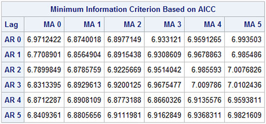
The model selection procedure ends up with an AR(1) model (see Output 7.10). This is seen as the corrected Akaike Information Criterion attains the smallest value (the optimal in this situation) 6.77 for AR 1 and MA 0.

Output 7.10: Values of the Information Criterion for Many Candidate Models

The estimated autoregressive parameter is .49 (Output 7.11), which is in line with the results in Chapter 5. The constant term is insignificant, which again indicates that the series of the number of cows has no trend.

Output 7.11: Estimated Autoregressive Parameter

The fit of the model is accepted by the portmanteau tests (Output 7.12). This sequence of tests provides no evidence of lack of fits. It is particularly noted that nothing happens to the series of portmanteau tests for lags 4, 8, or 12, where an eventual seasonality could lead to model deficits.

Output 7.12: Portmanteau Tests for Cross-Correlations of Residuals

PROC VARMAX Applied to the Series of Milk Production

For the milk production series, a seasonal component is clear from the results of Chapters 2–5, where quarterly dummies are included in the models. In PROC VARMAX, such dummies are easily coded inside the procedure application by an NSEASON=4 option to the MODEL statement (Program 7.8). This specification of the seasonality is easier than the user-specified dummy variables in Chapters 2–5.

Program 7.8: Model Selection for the Differenced Milk Production Series

The model selection by PROC VARMAX ends up with an MA(4) model. The estimated parameters are numerically large (Output 7.13), and the portmanteau test rejects the model (Output 7.14) for the smaller lags.

Output 7.13: Estimated Parameters for an MA(4) Model

Output 7.14: Portmanteau Tests for Cross-Correlations of Residuals from an MA(4) Model

The problem might be that something went wrong in the estimation algorithm, or perhaps, as is more likely, the model overfits because of the large number of parameters in the MA(4) model. This happens in some situations, especially when you try to fit a complicated model including moving average terms.

A Simple Moving Average Model of Order 1

If the model is explicitly stated as a simple MA(1) model, as in Program 7.9, the estimation is much more successful.

Program 7.9: Estimation of an AR(1) Model for the Differenced Milk Production Series

The fitted model has a single moving average parameter, which is significant (Output 7.15). The estimated parameter value MA1_1_1 = .44 (that is, the parameter θ₁) is positive. The model is formulated for the differenced series of milk production, Δy_t, which is the change in the milk production to one quarter from the previous quarter. If the seasonal dummies are left out, the model is expressed as follow:

Δy_t = ε_t − 0.44 ε_{t − 1}

Here, ε_t denotes the errors. This tells that if the milk production suddenly decreases (that is, if ε_t−1 is negative), the production will rise by − 0.44 ε_t−1 in the next quarter. A simple explanation could be that if some milk production for some reason is reported too late for one quarter, then this produced milk is included in the figures for the following quarter. In fact, an MA(1) model is often seen for time series that are differenced before identifying ARMA models.

Output 7.15: Estimated Parameters of an MA(1) Model for the Differenced Milk Production Series

The estimated constant, 1170.2, is positive (see Output 7.15). In the model, this constant represents the quarterly rise in milk production because of the upward trend in the series. Note, however, that the numbering of the quarters are in the order that the quarters appear in the data set. So the numbering does not necessarily begin with the first quarter of a year. Moreover, the reported value for the constant is not the estimated trend value for the series when seasonal dummies are present.

The numbering of the seasonal dummies does not correspond to the quarters within a calendar year. The numbering starts with the first available observation rather than simply the first observation in the data set. In this example, one observation is skipped because of the differencing; of course, the first observation misses a lagged observation. The first available observation is then the observation for the second quarter of 1998. This first available observation is taken as the reference. If the model had also included p autoregressive terms, p more observations would have been skipped.

By this numbering, the constant value CONST1 = 1170.2 is the constant for the second quarter. As the series is differenced, this positive value means that the milk production increases from the first quarter to the second quarter. The reported parameter SD_1_1 = − 3076.9 is then the coefficient to a dummy variable for the third quarter having the second quarter as the reference quarter. It then demonstrates that milk production tends to change by 1170.2 − 3076.9 = − 1906.7 from the second quarter to the third quarter, which is a notable reduction.

Similarly, the change from the third quarter to the fourth quarter is 1170.2 − 1343.7 = − 173.5, which says that the milk production is almost the same in the third quarter and the fourth quarter. The milk production increases by 1170.2 + 362.5 = 1532.7 from the fourth quarter of the year to the first quarter of the following year. This increase is almost equal to the rise from the first quarter to the second, which was the basic quarter in the model. This last conclusion is because the last estimated seasonal parameter SD_1_3 = 362.5 is insignificant, p = .11

The model then gives four derived average quarterly changes in the produced quantity of milk. The sum of these four numbers is 1170.2 − 1906.7 − 173.5 + 1532.7 = 622.7. This rather small positive value is then the estimated annual increase in milk production.

The model fit is accepted, as can be seen by the portmanteau tests’ having large p-values (Output 7.16).

Output 7.16: Portmanteau Tests for Autocorrelations of Residuals

This example demonstrates the strength of moving average models. An MA(1) model is seen to fit the time series very well. In fact, an autoregressive model must have the order 3 (that is an AR(3) model) in order to give the same fit for this data series when judged by portmanteau tests.

A drawback of a moving average model is that it is a bit harder to understand than an autoregressive model. In an autoregressive model, the terms are lagged values of the series itself and not of the error terms as in moving average models. But as explained above, it is at any rate possible to give a natural interpretation of MA models for differenced series.

In later chapters, this series for milk production is combined with the series for the number of cows to find a bivariate model. In order to do so, you will find that it is a good idea to start with similar univariate models for the two series.

Conclusion

It is good practice to start by studying the individual univariate time series before you try to establish multivariate models for their joint behavior. This chapter has demonstrated how to perform such analyses by PROC VARMAX, using four individual time series: the wage series, the price series, the milk production series, and the number-of-cows series. These series are applied in many chapters of this book. The results resemble the results obtained by other strategies for the analysis.

PROC VARMAX is used mainly for analysis of multivariate time series. But, as seen, PROC VARMAX is also useful for the analysis of univariate series. In later chapters, the interdependence between the wage and price series, and between the milk production and the number-of-cows series, is analyzed with PROC VARMAX.