
5 Performance
Performance is a very important topic when dealing with any database setup. One of the main reasons to use a cluster over a nonclustered database is the ability to get better performance and scalability compared to using a database that is confined to a single host. This chapter discusses many of the concepts related to performance and scalability, as well as how to ensure that you get the maximum from your MySQL Cluster setup.
Before we get into performance tuning, we need to discuss what performance means, as it can have different meanings to different people. Many different metrics can go into measuring performance and scalability, but the overall definition we use in this book is “ensuring that every client’s needs are satisfied as quickly as possible.” Beyond this definition, we can talk about many other related topics as well, such as response time, throughput, and scalability.
Response time indicates how long someone has to wait to be served. There are some different metrics based on this that are worth monitoring. First is maximum response time, which indicates how long anyone has to wait in the worst-case scenario. The second is the average response time, which is useful for knowing what the average response time is. Keep in mind that response time normally includes two different pieces of the time for a response: wait time and execution time. Wait time, or queue time, is how long the client has to block (that is, wait in a queue for access) before execution can begin. This wait occurs normally due to lock contention. Execution time is the amount of time actually spent running (that is, executing) statements.
Throughput is a metric that measures how many clients and requests you serve over some time period. Typically you might see this measured as queries per second or transactions per minute.
Finally, scalability is how well the previous two values can be maintained as the overall load increases. This increase in load might be tied to the number of database users, or it could possibly be independent of that. Sometimes, multiple dimensions of load increase at the same time. For example, as the number of users increases, the amount of data and the number of queries may both increase. This is often one of the hardest pieces to be sure of, due to the fact that it can be difficult to simulate the exact effects of these increases without them actually occurring.
MySQL Cluster has a very different impact on the concepts of response time, throughput, and scalability than a normal single-system, disk-based database, such as MyISAM or InnoDB.
Response time with MySQL Cluster is quite commonly worse than it is with the traditional setup. Yes, response time is quite commonly worse with clustering than with a normal system. If you consider the architecture of MySQL Cluster, this will begin to make more sense. When you do a query with a cluster, it has to first go to the MySQL server, and then it goes to data nodes and sends the data back the same way. When you do a query on a normal system, all access is done within the MySQL server itself. It is clearly faster to access local resources than to read the same thing across a network. As discussed later in this chapter, response time is very much dependant on network latency because of the extra network traffic. Some queries may be faster than others due to the parallel scanning that is possible, but you cannot expect all queries to have a better response time. So if the response time is worse, why would you use a cluster? First, response time isn’t normally very important. For the vast majority of applications, 10ms versus 15ms isn’t considered a big difference. Where MySQL Cluster shines is in relation to the other two metrics—throughput and scalability.
Throughput and scalability are generally much better with clustering than in a single-system database. If you consider the most common bottlenecks of the different systems, you can see why. With a single-system database, you almost always bottleneck on disk I/O. As you get more users and queries, disk I/O generally becomes slower due to extra seeking overhead. For example, if you are doing 1Mbps worth of access with one client, you might only be able to do 1.5Mbps with two and only 1.75Mbps with three clients. MySQL Cluster is typically bottlenecked on network I/O. Network traffic scales much better with multiple users. For example, if you are transferring 1Mbps with one client, you can do 2Mbps with two clients, 3Mbps with three clients, and so on. You start to have problems only when you near the maximum possible throughput. This allows you to scale the system relatively easily until you start to reach network limits, which are generally are quite high.
Benchmarking is a tool that, when used correctly, can help you plan for scalability, test throughput, and measure response time. When used incorrectly, benchmarking can give you a very wrong impression of these things.
In a good benchmark, you want to simulate your production environment as closely as possible. This includes things such as hardware available, software being used, and usage patterns.
The following sections describe some common problems with benchmarks.
When doing a benchmark, you need to have the same amount of data you plan on having in the system. Doing a benchmark with 50MB of data when you plan on having 10GB in production is not a useful benchmark.
If you are generating data, you need to make sure it isn’t too random. In real life, most data has patterns that cause more repeats of certain data than of other data. For example, imagine that you have a set of categories for something. In real life, certain categories are likely to be much more common than other categories. If you have exactly the same distribution of these in your generated data, this can influence the benchmark.
Using inaccurate data access patterns is similar to using a data set that is not representative, but it relates to data access instead. For example, if in your benchmark you are searching for “Latin dictionary” as commonly as “Harry Potter,” you will see different effects. Some things are much more commonly accessed than others, and your benchmarks need to take that into account.
There are two ways failing to consider cache effects can affect your benchmarking. First, you can run a benchmark that makes overly heavy use of caches. For example, if you run just the same query over and over, caching plays a very big role in it. Second, you can do completely different things over and over, which reduces the effectiveness of caches. This relates to the previously mentioned concept of data access patterns. “Harry Potter” would most likely have a high cache hit rate, but “Latin dictionary” wouldn’t make as much use of the cache, and this can be difficult to measure in benchmarks.
In order for a benchmark to be accurate, it needs to reflect the number of users who will be accessing your system. A very common problem with MySQL Cluster benchmarks is attempting to benchmark with only a single user (which MySQL Cluster is quite poor at due to bad response time, but it has great scalability and throughput).
Now that you know some of the problems with benchmarking, how can you work around them? One of the easiest ways is to benchmark against your actual application. For some application types, such as web applications, this is very easy to do. Two commonly used web benchmarking applications that are available for free are httperf (www.hpl.hp.com/research/linux/httperf/) and Microsoft Web Application Stress Tool (www.microsoft.com/technet/archive/itsolutions/intranet/downloads/webstres.mspx). For some application types, such as embedded applications, benchmarking is more difficult, and you may need to create a tool yourself.
The other solution is to use a benchmarking tool that can more closely mimic your application. Two tools in this category are Super Smack (http://vegan.net/tony/supersmack/) and mybench (http://jeremy.zawodny.com/mysql/mybench/). With both of these tools, you can more accurately represent what the query/user/data patterns are for your application. They require quite a bit of customization, but they can help you avoid some of the common pitfalls.
Indexes are extremely important in MySQL Cluster, just as they are with other database engines. MySQL Cluster has three different types of indexes: PRIMARY KEY indexes, UNIQUE hash indexes, and ordered indexes (T-tree).
The data in MySQL Cluster is partitioned based on a hash of the PRIMARY KEY column(s). This means the primary key is implemented through a hash index type. A hash index can be used to resolve queries that are used with equals but cannot be used for range scans. In addition, you need to use all of a PRIMARY KEY column and not just part of it.
The following is an example of queries that could use the PRIMARY KEY column:
SELECT * FROM tbl WHERE pk = 5;
SELECT * FROM tbl WHERE pk = 'ABC' OR pk = 'XYZ';
The following are examples of queries that will not use the PRIMARY KEY index:
SELECT * FROM tbl WHERE pk < 100;
SELECT * FROM tbl WHERE pk_part1 = 'ABC';
The first of these examples will not use the PRIMARY KEY index because it involves a range with less than and not a straight equality. The second example assumes that you have a two-part primary key, such as PRIMARY KEY (pk_part1, pk_part2). Because the query is using only the first half, it cannot be used.
Using the primary key is the fastest way to access a single row in MySQL due to the fact that your tables are partitioned on it.
Remember that when you declare a primary key in MySQL Cluster, by default you get both the PRIMARY KEY hash index and an ordered index, as described in the following section. It is possible to force the primary key to have only a hash index if you aren’t going to be doing range lookups. Here is how you implement that:
PRIMARY KEY (col) USING HASH
UNIQUE hash indexes occur whenever you declare a UNIQUE constraint in MySQL Cluster. They are implemented through a secondary table that has the column you declared UNIQUE as the primary key in the table along with the primary key of the base table:
CREATE TABLE tbl (
Id int auto_increment,
Name char(50),
PRIMARY KEY (id),
UNIQUE (Name)
);
This gives you a hidden table that looks like the following:
CREATE TABLE hidden (
Name_hash char(8),
Orig_pk int,
PRIMARY KEY (name_hash)
);
These tables are independently partitioned, so the index may not reside on the same node as the data does. This causes UNIQUE indexes to be slightly slower than the PRIMARY KEY, but they will still be extremely fast for most lookups.
An ordered index in MySQL Cluster is implemented through a structure called a T-tree. A T-tree works the same as a B-tree, but it is designed for use with in-memory databases. The two primary differences are that a T-tree is generally much deeper than a B-tree (because it doesn’t have to worry about disk seek times) and that a T-tree doesn’t contain the actual data itself, but just a pointer to the data, which makes a T-tree take up less memory than a similar B-tree.
All the queries that could be resolved with a B-tree index can also be resolved by using a T-tree index. This includes all the normal range scans, such as less than, between, and greater than. So if you are switching an application from MyISAM or InnoDB to MySQL Cluster, it should continue to work the same for query plans.
A T-tree itself is partitioned across the data nodes. Each data node contains a part of the T-tree that corresponds to the data that it has locally.
The MySQL optimizer uses various statistics in order to decide which is the most optimal method for resolving a query. MySQL particularly makes use of two different values: the number of rows in the table and an estimate of how many rows will match a particular condition.
The first value is approximately the number of rows in a table. This is important for deciding whether MySQL should do a full table scan or use indexes. MySQL Cluster can provide this value to the MySQL optimizer, but it doesn’t necessarily have to do so. The problem with retrieving this data from the data nodes for each query being executed is that it adds a bit of extra overhead and slightly degrades the response time of your queries. There is therefore a way to turn off the fetching of the exact number of rows. The MySQL server setting ndb_use_exact_count controls whether to do the retrieval. If the MySQL server doesn’t retrieve an exact value, it will always say there are 100 rows in the table.
Due to the distributed and in-memory natures of the MySQL storage engine, it is almost always best to use an index, if possible. In most cases, you want to turn off the ndb_use_exact_count variable to gain performance because it favors index reads.
As a side note, the ndb_use_exact_count variable has an impact on the following simple statement:
SELECT count(*) FROM tbl;
If you are familiar with the other storage engines, you know that MyISAM has an optimization to speed this up, whereas InnoDB doesn’t. The ndb_use_exact_count setting affects NDB in a similar manner: If it is on, it works like MyISAM, but if it is off, it works like InnoDB. The nice thing is that you can set this on a per-connection basis, which allows you to do something such as the following:
mysql> set ndb_use_exact_count = 1;
Query OK, 0 rows affected (0.00 sec)
root@world~> SELECT count(*) FROM Country;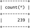
1 row in set (0.01 sec)
mysql> set ndb_use_exact_count = 0;
Query OK, 0 rows affected (0.01 sec)
The other value that MySQL uses is an estimation of how many rows will match against a particular index lookup. MySQL Cluster currently isn’t able to calculate this value. It always estimates that 10 rows will match. If you combine this with the preceding rule of 100 rows, you see that MySQL will always use indexes, which is good with MySQL Cluster. Where the problem comes with this is where MySQL has choices between multiple indexes. The following query shows the problem:
SELECT * FROM tbl WHERE idx1 = 5 AND idx2 = 10;
MySQL Cluster tells MySQL that both idx1 and idx2 will retrieve the same number of rows (10). However, normally this might not be true; one of the indexes is typically more selective than the other. In this case, because MySQL Cluster doesn’t have the information available, you have to tell MySQL which one is better. To tell it which one, you should use a USING INDEX clause in the SELECT statement. So if the second index is more selective, you write a statement similar to the following:
SELECT * FROM tbl USING INDEX (idx2) WHERE idx1 = 5 AND idx2 = 10;
MySQL 5.1 will have the ability for NDB to estimate the rows that will match when using an index. This will prevent you from having to tell MySQL which index is more selective in most cases.
Query execution in MySQL Cluster can use a couple different methods. Which method is used makes a large difference in the response time of a query.
When MySQL receives a query, many different steps occur before you receive the results. The path is roughly laid out like this:
1. Receive query over network
2. Check query cache
3. Parse query
4. Check permissions
5. Optimize query:
a. Query transformations
b. Decide the order in which to read the tables
c. Decide on index use
d. Decide which algorithms to use for retrieval
6. Query execution:
a. Retrieval of data, based on preceding plan
b. Apply expressions to retrieved data
c. Sort data as necessary
7. Return results back to client
MySQL Cluster comes into play in step 5(a). MySQL Cluster is the storage engine that does the actual physical retrieval of data. All the other steps are done on the MySQL server side and work the same as with other storage engines. Before we talk further about this, we need to discuss the one other step that is affected as well: the query cache.
The query cache is a special cache that exists in MySQL to cache a query and a result set. If someone sends exactly the same query again, MySQL can return the result set directly from the cache instead of having to execute it again. When the data in a table changes, the query cache invalidates all the queries that involve that table, in order to prevent serving stale data. This is generally how it works with MySQL, but it gets a bit more involved with MySQL Cluster.
First, the query cache doesn’t work at all with MySQL Cluster version 4.1. This shortcoming has been fixed in MySQL 5.0, but it does work slightly differently. The reason it works differently is that data can change in many different MySQL servers without the other MySQL servers being aware of the changes. If the server isn’t aware of changes, then it can’t invalidate the cache, which leads to incorrect results.
When you have the query cache on and NDB enabled, MySQL creates an extra thread internally to periodically check what tables have been changed. Doing this check causes a bit of extra overhead for the MySQL server. Due to this extra overhead, you need to keep a few things in mind.
First, you should ensure that you are getting good use of the query cache. You can monitor the query cache status variables in order to see what percentage of them are using the cache:
mysql> SHOW STATUS LIKE 'Qcache%';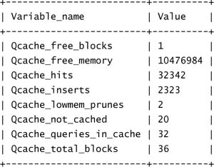
8 rows in set (0.00 sec)
The important variables to monitor are Qcache_hits, Qcache_inserts, and Qcache_not_cached. You need to ensure that Qcache_hits is generally larger than the other two values added together (which is the query cache miss rate).
The second thing you can do is change a value called ndb_check_cache_time. This variable tells how many seconds MySQL Cluster should wait between checking for data changes that were made on another MySQL server. The default setting is 0, which means MySQL Cluster will constantly be checking. Increasing this variable greatly reduces the overhead, but, in theory, it means there is a chance that the query cache will return slightly incorrect data. For example, it might return incorrect data if someone changes data on one server and any queries until the next server checks for that change return incorrect data. Whether this is okay depends entirely on the application. Normally any setting above 1 wouldn’t be needed because the server checks only once per second for invalidations.
MySQL Cluster has four different methods of retrieving data with different performance characteristics: primary key access, unique key access, ordered index access, and full table scans.
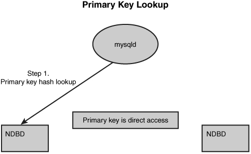
When a query is going to use the primary key, it does so using a normal hash lookup. The MySQL server forms a hash of the primary key, and then, using the same algorithm for partitioning, it knows exactly which data node contains the data and fetches it from there, as shown in Figure 5.1. This process is identical, no matter how many data nodes are present.
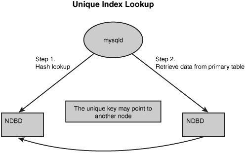
When a query is going to use a unique key, it again does a hash lookup. However, in this case, it is a two-step process, as shown in Figure 5.2. The query first uses a hash on the UNIQUE value to look up the PRIMARY KEY value that corresponds to the row. It does this by using the value as the primary key into the hidden table. Then, when it has the primary key from the base table, it is able to retrieve the data from the appropriate place. For response time purposes, a UNIQUE access is approximately double the response time of a primary key lookup because it has to do two primary key lookups to get the row.
To access an ordered index, the MySQL server does what is a called a parallel index scan, as shown in Figure 5.3. Essentially, this means that it has to ask every single data node to look through the piece of the index that the data node has locally. The nodes do this in parallel, and the MySQL server combines the results as they are returned to the server from the data nodes.
Due to the parallel nature of the scanning, this can, in theory, have a better response time than doing a local query. This is not always true, however, as it depends on many different things.
An ordered index scan causes more network traffic and is more expensive than a PRIMARY KEY or UNIQUE KEY lookup. However, it can resolve a lot of queries that cannot be resolved by using a hash lookup.
The final method for resolving a query is through the use of a full table scan. MySQL Cluster can do this in two different ways, depending on the version and startup options you use for the MySQL server:
![]() Full table scan without condition pushdown—This first option is the slower, less efficient method. In this method, all the data in the table is fetched back to the MySQL server, which then applies a
Full table scan without condition pushdown—This first option is the slower, less efficient method. In this method, all the data in the table is fetched back to the MySQL server, which then applies a WHERE clause to the data. As you can imagine, this is a very expensive operation. If you have a table that is 2GB in size, this operation results in all 2GB of data crossing the network every time you do a full table scan. This method is the only one available in MySQL 4.1. It is also the default method in MySQL 5.0.
![]() Full table scan with condition pushdown—There is an option in MySQL 5.0 called
Full table scan with condition pushdown—There is an option in MySQL 5.0 called engine_condition_pushdown. If this option is turned on, the MySQL server can attempt to do a more optimized method for the full table scan. In this case, the WHERE clause that you are using to filter the data is sent to each of the data nodes. Each of the data nodes can then apply the condition before it sends the data back across the network. This generally reduces the amount of data being returned and can speed up the query over the previous method by a great deal. Imagine that you have a table with 2 million rows, but you are retrieving only 10 rows, based on the WHERE condition. With the old method, you would send 2 million rows across the network; with the new method, you would only have to send the 10 rows that match across the network. This reduces the network traffic by almost 99.9999%. As you can imagine, this is normally the preferred method.

To enable the engine_condition_pushdown option, you need to set it in the MySQL configuration file:
[mysqld]
ndbcluster
engine_condition_pushdown=1
You can also set it dynamically by using either the SET GLOBAL or SET SESSION command, like this:
SET SESSION engine_condition_pushdown=1;
SET GLOBAL engine_condition_pushdown=0;
SET GLOBAL applies to all future connections. SET SESSION applies to only the current connection. Keep in mind that if you want to have the value survive across a MySQL server, you should restart and then change the configuration file.
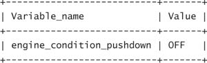
You can verify that the engine_condition_pushdown variable is currently on by using the SHOW VARIABLES command:
mysql> show variables like 'engine%';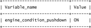
1 row in set (0.00 sec)
After this variable has been set, you can ensure that it is actually working by using the EXPLAIN command. If it is working, you see the Extra option called “Using where with pushed condition”:
mysql> EXPLAIN SELECT * FROM country WHERE name LIKE '%a%'G
*************************** 1. row ***************************
id: 1
select_type: SIMPLE
table: country
type: ALL
possible_keys: NULL
key: NULL
key_len: NULL
ref: NULL
rows: 239
Extra: Using where with pushed condition
1 row in set (0.00 sec)
The EXPLAIN command is the key to knowing which of the access methods are being used and how MySQL is resolving your query.
To use EXPLAIN, all you have to do is prefix your SELECT statement with the keyword EXPLAIN, as in the following example:
Note
Note that these examples use the world database, which is freely available from the documentation section of http://dev.mysql.com.
If you want to try out these exact examples, you can download and install the world database and switch all the tables to NDB by using ALTER TABLE. Remember to create the database world on all SQL nodes.
mysql>EXPLAIN SELECT * FROM Country, City WHERE Country.capital = City.id
AND Country.region LIKE 'Nordic%'G
*************************** 1. row ***************************
id: 1
select_type: SIMPLE
table: Country
type: ALL
possible_keys: NULL
key: NULL
key_len: NULL
ref: NULL
rows: 239
Extra: Using where
*************************** 2. row ***************************
id: 1
select_type: SIMPLE
table: City
type: eq_ref
possible_keys: PRIMARY
key: PRIMARY
key_len: 4
ref: world.Country.Capital
rows: 1
Extra:
2 rows in set (0.00 sec)
There is a lot of information here, so let’s examine what it all means.
The first significant thing we need to examine is the order in which the rows come back. The order is the order in which MySQL is going to read the tables. This order does not normally depend on the order in which they are listed in the query. For inner joins and some outer joins, MySQL rearranges the tables into any order it feels will make your query faster.
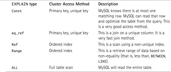
The next thing that is important is the Type column. It tells how MySQL is going to read the table. This ties in to the previous section about table access methods. Some of the possible retrieval types and what they correspond to for MySQL Cluster are listed in Table 5.1.
The next two columns in EXPLAIN are possible_keys and key. These columns indicate which indexes MySQL is using and also which indexes it sees are possible but decides not to use to resolve your query. Due to the lack of index statistics, as mentioned previously in this chapter, you might consider suggesting one of the other possible indexes with USE INDEX to see if it is any faster with a different one.
The next column of significance is the rows column. This column tells how many rows MySQL thinks it will have to read from the table for each previous combination of rows. However, this number generally isn’t all that accurate because NDB does not give accurate statistics to MySQL. Normally, if you are using an index, you will see 10 listed as the rows, regardless of how many rows actually match. If you are doing a full table scan, you will also see 100 if ndb_use_exact_count is turned off. If ndb_use_exact_count is enabled, the rows column correctly gives the number of rows in the table that need to be scanned.
The final column listed is the Extra column. This column can list any additional information about how the query is going to be executed. The first important value that can show up here is Using where with pushed condition. As mentioned previously, this means that NDB is able to send out the WHERE condition to the data nodes in order to filter data for a full table scan. A similar possible value is Using where. This value indicates that the MySQL server isn’t able to send the filtering condition out to the data nodes. If you see this, you can attempt to get the MySQL server to send it out in order to possibly speed up the query.
The first thing you can do is ensure that the engine_condition_pushdown variable is set. You can view whether it is set by using the SHOW VARIABLES option:
mysql> EXPLAIN SELECT * FROM Country WHERE code LIKE '%a%'G
*************************** 1. row ***************************
id: 1
select_type: SIMPLE
table: Country
type: ALL
possible_keys: NULL
key: NULL
key_len: NULL
ref: NULL
rows: 239
Extra: Using where
1 row in set (0.14 sec)
mysql> show variables like 'engine_condition_pushdown';
1 row in set (0.01 sec)
root@world~> set session engine_condition_pushdown=1;
Query OK, 0 rows affected (0.00 sec)
mysql> explain SELECT * FROM Country WHERE code LIKE '%a%'G
*************************** 1. row ***************************
id: 1
select_type: SIMPLE
table: Country
type: ALL
possible_keys: NULL
key: NULL
key_len: NULL
ref: NULL
rows: 239
Extra: Using where with pushed condition
1 row in set (0.00 sec)
The second method you can attempt is to rewrite the query into something that can be pushed down. In order to be able to push down a WHERE condition, it has to follow these rules:
![]() Any columns used must not be used in expressions (that is, no calculations or functions on them).
Any columns used must not be used in expressions (that is, no calculations or functions on them).
![]() The comparison must be one of the supported types. Supported types include the following:
The comparison must be one of the supported types. Supported types include the following:
![]()
=,!=,>,>=,<,<=,IS NULL, and IS NOT NULL
![]() Combinations of the preceding types (for example,
Combinations of the preceding types (for example, BETWEEN, IN())
![]()
AND and OR are allowed.
The following is an example of how to rewrite a query to make use of the condition pushdown:
mysql> explain SELECT * FROM Country WHERE population < 1000/1.2 < 1000
OR code LIKE �%a%� G
*************************** 1. row ***************************
id: 1
select_type: SIMPLE
table: Country
type: ALL
possible_keys: NULL
key: NULL
key_len: NULL
ref: NULL
rows: 239
Extra: Using where
1 row in set (0.09 sec)
mysql> explain SELECT * FROM Country WHERE population < 1000/1.2
OR code LIKE '%a%’ G
*************************** 1. row ***************************
id: 1
select_type: SIMPLE
table: Country
type: ALL
possible_keys: NULL
key: NULL
key_len: NULL
ref: NULL
rows: 239
Extra: Using where
1 row in set (0.00 sec)
Notice that in the second explain, the query was rewritten to put the population column used all by itself on one side. That allowed the condition to be pushed down, which will potentially enable the full table scan to be many times faster.
One of the most important factors when dealing with the response time of MySQL Cluster is network latency. The lower the network latency, the lower the response time.
Any operation that occurs within MySQL Cluster normally has numerous round trips across the network as messages are passed around between data nodes and the MySQL server. For example, during a transaction commit, NDB needs to do a two-phase commit procedure, which ensures that all the data nodes have the correct data (due to synchronous replication).
The number of operations performed during a two-phase commit is measured as follows:
Num. of Messages = 2 × Num. of Fragments ×(NoOfReplicas + 1)
Assume that you have four data nodes with NoOfReplicas set to 2. That gives us 2 × 4 × (2 + 1) = 24 messages. If we have a latency of .5ms between nodes, that gives us a total network time of 24 × .5 = 12ms. Reducing the latency by even a little bit will make a relatively large difference due the number of messages.
There are a few things to note with this. First, most operations do not involve so many messages. For example, a single primary key lookup results in just two messages: the request for the row and the return of the row. Network latency still plays a big part in response time, but the effects of changing the latency are smaller for some messages due to the smaller number of messages.
The second important concept to mention is message grouping. Because so many messages are being passed by MySQL Cluster in a highly concurrent environment, MySQL can attempt to piggyback messages on other ones. For example, if two people are reading data at the same time, even from different tables, the messages can be combined into a single network packet. Because of the way network communications work, this can improve throughput and allow for much more concurrency before the network becomes saturated by lowering the overhead for each message. The drawback of this grouping is that there is a slight delay before requests are sent. This slight delay causes a decrease in response time. In many cases, this is totally acceptable for the increase in throughput.
In some cases, the extra delay introduced by this isn’t useful. The two most common cases are when there isn’t a lot of concurrency and when response time is more important than throughput. In a situation of low concurrency, such as initial data imports, benchmarks that are being done with only a single thread, or little-used applications (for example, five queries per second), it makes sense to disable this optimization. The variable ndb_force_send can control this behavior. If this variable is turned off, MySQL Cluster groups together messages, if possible, introducing a slight response time decrease. If it is turned on, it attempts to group messages together, which should increase throughput.
In order to get the best response time and to increase throughput, the most important physical aspect is the network interconnect.
NDB currently supports three different connection methods, also called transports: TCP/IP, shared memory, and SCI. It is possible to mix different transports within the same cluster, but it is recommended that all the data nodes use the same transport among themselves, if possible. The default if you don’t specify is to use TCP/IP for all the nodes.
TCP/IP is by far the most common connection protocol used in NDB. This is due to the fact that it is the default and also is normally preconfigured on most servers. The management node always makes use of TCP/IP. It cannot use shared memory or SCI. Normally, the fact that it can’t use a high-speed interconnect should not be an issue because there isn’t very much data being transferred between the management node and others.
TCP/IP is available over many different mediums. For a base cluster in MySQL Cluster, Gigabit Ethernet would be the minimum recommended connection. It is possible to run a cluster on less than that, such as a 100MB network, but doing so definitely affects performance.
Generally, you want your networking hardware to be high quality. It is possible to get network cards that can do much of the TCP/IP implementation. This helps to offload CPU usage from your nodes, but it will generally lower network latency slightly. Each little bit that you can save on network latency helps.
If you are looking for even higher performance over TCP/IP, it is possible to use some even higher network or clustering interconnects. For example, there is now 10GB Ethernet, which may increase performance over Gigabit Ethernet. There are also special clustering interconnects, such as Myrinet, that can make use of the TCP/IP transport as well. Myrinet is a commonly used network transport in clusters. Because it can use TCP/IP, it can be used with MySQL Cluster as well.
When examining the more expensive options, we highly recommend that you acquire test hardware if possible. Many of these interconnects cost many times what commodity hardware, such as Gigabit Ethernet, costs. In some applications, interconnects can make a large performance difference, but in others, they may not make a very great difference. If the performance isn’t much better, it might be wiser to spend more of your budget on something else, such as more nodes.
MySQL Cluster can make use of shared memory connections. Shared memory connections are also referred to as the SHM transport. This type of connection works only when two nodes reside on the same physical machine. Most commonly, this is between a MySQL server and a data node that reside locally, but it can be used between data nodes as well.
Generally, shared memory connections are faster than TCP/IP local connections. Shared memory connections require more CPU, however, so they are not always faster due to CPU bottlenecks. Whether a CPU bottleneck decreases performance is highly application specific. We recommend that you do some benchmark testing between shared memory and TCP/IP local connections to see which is better for your particular application.
In order to use the NDB shared memory transport, you need to ensure that the version you are using has the transport compiled in. Unfortunately, not all the operating systems that support MySQL Cluster contain the necessary pieces to support shared memory connections. If you are compiling yourself, you need to compile MySQL with the option --with-ndb-shm.
When you are sure that your platform contains the transport, you need to configure MySQL Cluster to use it. There are two different ways to configure shared memory connections. The first option is designed to allow for more automatic configuration of shared memory. The second requires manual configuration but is a bit more flexible.
The first option is controlled by a startup option for the MySQL server called ndb-shm. When you start mysqld with this option, it causes mysqld to automatically attempt to use shared memory for connections, if possible. Obviously, this works only when connecting to local data nodes, but you can run with this option regardless of whether there are any local data nodes.
The second option is to set up shared memory by putting it in the cluster configuration file (normally config.ini). For each shared memory connection you want, you need to add a [SHM] group. The required settings are the two node IDs involved and a unique integer identifier. Here is an example:
[SHM]
NodeId1=3
NodeId2=4
ShmKey=324
NodeId1 and NodeId2 refer to the two nodes you want to communicate over shared memory. You need a separate [SHM] section for each set of two nodes. For example, if you have three local data nodes, you need to define three [SHM] sections (that is, 1–2, 2–3, and 1–3).
You may want to define some optional settings as well. The most common setting is called ShmSize. It designates the size of the shared memory segment to use for communication. The default is 1MB, which is good for most applications. However, if you have a very heavily used cluster, it could make sense to increase it a bit, such as to 2MB or 4MB.
Scalable Coherent Interface (SCI) is the final transport that MySQL Cluster natively supports. SCI is a cluster interconnect that is used commonly for all types of clusters (not only MySQL Cluster). The vendor that provides this hardware is called Dolphin Interconnect Solutions, Inc. (www.dolphinics.com).
According to MySQL AB’s testing, SCI normally gives almost a 50% reduction in response time for network-bound queries. Of course, this depends on the queries in question, but it generally offers increased performance.
There are two ways you can use this interconnect. The first is through the previously mentioned TCP/IP transport, which involves an interface called SCI Sockets. This interface is distributed by Dolphin Interconnect Solutions and is available for Linux only. This is the preferred method for use between the MySQL server and data nodes. From a MySQL Cluster perspective, the network is just set up to use normal TCP/IP, but the SCI Sockets layer translates the TCP/IP into communication over SCI. For configuration information, see the SCI Sockets website, at www.dolphinics.com.
The second way to use SCI is through the native NDB transport designed for it, which uses the native SCI API. To make use of this, you need to compile MySQL Cluster with support for it, using the option --with-ndb-sci. This is the normal method to use between data nodes as it is normally faster than using SCI Sockets.
In order to use the native SCI transport, you need to set up your cluster configuration file (config.ini) with the connection information. For each SCI connection, you need to create a section called [SCI]. The required options to use under this option are described in the following sections.
The two options NodeId1 and NodeID2 define which nodes are going to be involved in this connection. You need to define a new group for each set of nodes. For example, if you have four nodes that all use SCI, you need to define 1–2, 1–3, 1–4, 2–3, 2–4, and 3–4. Imagine if you have a large number of data nodes (such as eight or more): You might have quite a few sections. The actual number of sections required is the combination of the number of data nodes, taken two at a time (nC2).
The values Host1SciId0, Host1SciId0, Host2Sci0, and Host2Sci1 designate which SCI devices to use. Each node needs to have at least one device defined to tell it how to communicate. You can, however, define two devices for each node. SCI supports automatic failover if you have multiple SCI communication devices installed and configured to use. The actual ID number is set on the SCI card.
The optional parameter SharedBufferSize specifies how much memory to devote on each end for using SCI. The default is 1MB, which should be good for most applications. Lowering this parameter can potentially lead to crashes or performance issues. In some cases, you might get better performance by increasing this parameter to slightly larger sizes.
The following is an example of a single entry (remember that you will quite often need more than just one):
[SCI]
NodeId1=5
NodeId2=7
Host1SciId0=8
Host2SciId0=16
It is possible to implement new transports relatively easily due to the separation of the transport layer from the logical protocol layer. Doing so requires writing C++ code. Although most people do not have to do this, it might prove advantageous in some cases. How to actually do it is beyond the scope of this book, but to get started, we would recommend that you do two things. First, you can refer to the source code in the directory called ndb/src/common/transporter, which is part of the MySQL source code distribution, and pay close attention to the class Transporter in transporter.hpp. Second, if you need assistance, you can ask on [email protected] or through your support contract, if you have one.