2
The Sphere of Semantics
2.1. Combinatorial semantics
Far from the theoretical or psycholinguistic controversies about the role and manner in which humans combine different resources of linguistic information to construct meaning in a sentence, it is generally accepted that the lexicon and syntax play a non-negligible role in this process1. Because these two sources of information are not always sufficient, high-level semantic constraints are indispensable for distinguishing different possible interpretations of the same syntactic structure. For example, the subject and the object of a sentence can play different semantic roles. Sometimes, the subject is the direct cause of an event that is voluntary or not (e.g. John writes), or the indirect or unconscious cause (e.g. it is raining). Sometimes, it is the subject that is affected by the action expressed by the verb (as in, John dies).
2.1.1. Interpretive semantics
At the start of the 1960s, Fodor and Katz [FOD 64] proposed enriching syntactic structures constructed in the form of trees with a semantic analysis.
Interpretive semantics establishes a clear distinction between aspects of interpretation that are founded on linguistic knowledge and aspects of interpretation that are derived from knowledge about the world. According to this theory, it is this distinction that makes it possible to draw the boundary between semantics and pragmatics. It assumes that semantics must account for all of the possible interpretations of a given sentence independent of the limits imposed by knowledge about the world. The objectives of this theory can be summarized by the following points:
- – to determine the number and content of possible interpretations of a sentence;
- – to detect semantic anomalies;
- – to decide whether there are paraphrase relations between two sentences;
- – to indicate all other semantic properties that play a role in this capacity.
According to Katz and Fodor, semantics is based on two fundamental components: a dictionary and projection rules. In this context, it is assumed that grammatical analysis is pre-existing.
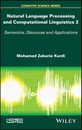
The role of the dictionary is to provide information about the parts of speech (noun, verb, adjective, etc.) as well as a description of the role played by the words in the semantic interpretation in the form of marker or features such as: (±human), (±concrete) and (±animated). The lexicon also contains so-called lexical redundancy rules that represent the relations between these features. For example, the rule (+human) → (+animated) indicates that everything that belongs to the class of humans also belongs to the class of animated beings.
For example, the word pig can have the description given in Figure 2.1.
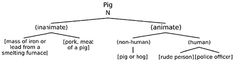
Figure 2.1. Description of the word pig according to the model in [FOD 64]
In Figure 2.1, the syntactic categories are represented without parentheses, the semantic categories are in parentheses, and the semantic features are in square brackets.
The projection rules define the way in which the different aspects of the meaning of a lexical item can be combined in the framework of grammatical constituents. In doing so, they indicate how the set of sentences encountered by a locutor are projected on the infinite set of grammatical sentences in language.
To illustrate these ideas, consider the following sentence as an example: the man drives the colorful car2. In this seemingly simple sentence, there are three cases of lexical ambiguity. The first concerns the word to drive which can be interpreted in at least four ways, including3: to operate a vehicle, to cause someone or something to move, to travel, and to motivate, compel or force. The second word, car, can in turn have at least three different meanings: automobile, conveyance for passengers on a cable railway, and passenger compartment of an elevator. Another ambiguity concerns the word colorful, which can have at least two different interpretations: that which has one or several colors, or that which is vivid or lively. In theory, the number of possible interpretations of a sentence is equal to multiplying the number of interpretations for each ambiguous word. In this case, this means there are 24 interpretations: 4*3*2. Projection rules intervene here and exclude some combinations through selective restrictions that specify the necessary and sufficient conditions. For example, the word to drive in the sense to motivate has a selective restriction that limits its occurrence to animated objects (to motivate your friend, to motivate your fellow citizens, etc.) and it therefore cannot be employed with an inanimate object like car. Similarly, the adjective colorful in its figurative sense meaning vivid and lively requires a noun that designates an abstract entity (e.g. ideas, style, expression) and cannot qualify a noun that designates a concrete entity like car.
The work by [KAT 64] concluded that all of the information necessary for applying projection rules can be found in the deep structure. In other words, the transformation operations do not affect the meaning of the final sentence. Known today as the Katz–Postal hypothesis, this conclusion has been supported by several observations. First of all, the rules of the passive modify the grammatical relations of the sentence. It seemed logical to apply projection rules to a structural level that pre-exists the application of these rules: deep structure. Second, discontinuity phenomena were typically created by transformation rules whereas discontinuous deep structures that became continuous after transformations had never been observed. This was seen as an argument in favor of their interpretation at the deep level where the semantic unit is reflected by its syntactic continuity.
This perspective of the role of semantics is consistent with the standard theory by [CHO 57, CHO 65]. This theory stipulates the existence of formal rules for which the role is to generate sentence skeletons that are then lexically enriched by lexical insertion rules to create the deep structure. Finally, transformation rules are applied to the deep structure to produce surface structures such as negative, interrogative or passive structures. Thus, the role of semantics is to interpret the deep structure (hence the name interpretive semantics) which, after the transformations, receives a phonetic interpretation.
Later, Chomsky and his students began to recognize that certain properties in the surface structure like accentuation played a role in the semantic interpretation of the sentence, as in sentences [2.1] where the accent is marked by an apostrophe:
- – Mary bought her laptop at the store’. [2.1]
- – Mary bought her laptop’ at the store.
Although these two sentences are syntactically identical, they are not semantically equivalent: in the first sentence, the information is shared between the locutor and the recipient, whereas in the second sentence, only the locutor has the information in advance. Thus, the location of the accent, a surface pronunciation phenomenon, contributes to a change in the focus of the sentence and therefore a semantic change.
Using examples like [2.2a] and [2.2b], Jackendoff demonstrated that passive transformation plays a role in the interpretation of the sentence:
- a) Many arrows did not hit the target. [2.2]
- b) The target was not hit by many arrows.
The scope of many in [2.2] seems larger in sentence a than in sentence b. The word order, which is also a surface phenomenon, seems to play a semantic role. Consider sentences [2.3].
- a) John only reads books about politics. [2.3]
- b) Only John reads books about politics.
The scope of the quantifier only is not the same in sentences [2.3a] and [2.3b]. In the first case, it pertains to the object complement and in the second case, it concerns the subjects.
Most researchers from the interpretive school agreed with Chomsky that deep structure alone is not sufficient to provide all of the elements necessary for the interpretation of the sentence [CHO 71]. This new view of syntax and semantics is generally called Extended Standard Theory.
During the 1970s, Ray Jackendoff proposed a more complete model of interpretive semantics [JAC 72]. It consisted of a distributed model where there was no single semantic representation, but rather several types of rules that apply at several levels. Four components of meaning, each of which is derived from a group of interpretive rules, are distinguished: the functional structure, the modal structure, the table of coreference, and focus and presupposition.
The functional structure specifies the main propositional content of the sentence. It is determined by projection rules that apply to the deep structure. For example, to resolve the problem of the passive transformation shown in sentences [2.2], there are rules such as:
- – the subject of the deep structure of the phrase must be interpreted as the semantic agent of the verb;
- – the direct object of the deep structure must be interpreted as the semantic patient of the verb.
The modal structure specifies the scope of logical elements such as negation and quantifiers as well as referential properties like nominal groups. The following rule is given as an example: if logical element A precedes logical element B in the surface structure, then A must be interpreted as having a wider scope than B where the logical elements include quantifiers, negatives and some modal auxiliaries.
The table of coreference concerns the way in which elements like pronouns are considered to be coreferential with their antecedents. This was contrary to the dominant idea at the time, according to which sentences with anaphors were the result of a pronominalization transformation. Thus, sentence [2.4] is the result of the transformation:
- a) Frank thinks that Frank will succeed this year. [2.4]
- b) Franki thinks that he will succeed this year.
Thus, sentence [2.4a] is considered to be a transformation of [2.4b]. This explanation, although it is appealing, does not account for sentences with crossed coreferences such as the ones discovered by Emmon Bach [BAC 89]:
- – [The man who deserves itj]i will get [the prize he desires]j [2.5]
The existence of a reference from one nominal group to another, which in turn refers to the first one, involves an impossible deep structure: every anaphor can be found in the antecedent of another.
Focus and presupposition concern the distinction between the parts of the sentence that are considered to be new (providing new information) or those that are old.
Toward the end of the 1970s, ideas about deep structure and transformation began to give way to more functional approaches like in [BRE 82].
2.1.2. Generative semantics
Developed in the mid-1960s in response to the interpretive semantics of Fodor and Katz, generative semantics stipulates that the semantic component is generative while the syntactic component is interpretive. In other words, according to this approach, the role of the syntactic component is to provide appropriate structures to the meaning of the sentence that plays the role of deep structure through transformation operations (see the diagram in Figure 2.2). This approach is attributed jointly to several researchers including George Lakoff, James McCawley, Paul Postal and John R. Ross.
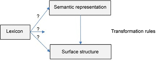
Figure 2.2. General diagram of the initial model of generative semantics
This amalgamation of syntax and semantics led to the formulation of three main hypotheses that are inherent in generative semantics. The first stipulates that deep structure as conceived by Chomsky in his book Aspects of the Theory of Syntax [CHO 65] does not exist. According to the second hypothesis, the initial representations of the derivations are logical. They are thus independent of language based on the hypothesis of a universal base. Finally, the derivation of a sentence is a connection between a semantic representation and a surface form.
Note that in Figure 2.3, the place and the way in which the lexicon intervenes in the derivation is controversial. Among others, [MCC 76] proposed a solution that treats lexical entries as semantic structures. For example, according to this approach, the verb to kill is derived from an abstract semantic representation: to cause to become not alive. This representation gives the following structure to the sentence John killed Mary. This deep structure is expressed semantically in terms of metalinguistics such as to cause, alive, etc.
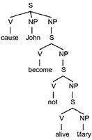
Figure 2.3. Semantic representation of the deep structure for: John killed Mary
To move from the deep structure to the surface structure, several predicate raising operations are carried out on the semantic tree. These operations make it possible to raise the verb from one embedded sentence to the next higher level, where it is attached to the verb in the sentence at that level. Thus, alive is raised to a higher level where it is attached to not. The result of this operation is given in Figure 2.4.
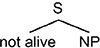
Figure 2.4. Result of a predicate raising operation
The successive application of such operations leads to a combination of the constituents to cause, to become, not and alive. Finally, generativists and interpretivists did not consider their respective theories as being cognitive models of the production or analysis of sentences. This led some linguists to conclude that the debate between the two camps had no point.
2.1.3. Case grammar
Proposed by Charles Fillmore at the end of the 1960s as a major modification to transformational grammar, case grammar quickly gained popularity, especially in the United States [FIL 68]. As in many other linguistic theories, there is no unified form of case grammar. In fact, Fillmore proposed several successive versions in the 1960s and 1970s [FIL 66, FIL 71, FIL 77].
Unlike classic cases observed in languages like Latin, Russian and Arabic, where the functions and/or semantic roles are signaled using suffixes, the cases proposed by Fillmore are more general and serve to model the relation between the verb, which plays the role of a logical predicate, and nominal groups in the sentence, which are treated like participants4. Two important properties are attributed to cases: they are universal and only a limited number exist.
The semantic representation obtained in this approach is considered to be the deep structure of the sentence. Thus, it is necessary to separate the grammatical functions (subject, object, etc.) and the cases that represent the underlying semantic relations between the participants in the situation evoked by the verbal predicate. For example, in sentences [2.6], John is considered to be an agent, although he has the same syntactic function in the surface forms of the sentence:
- (John subject/agent) hit Peter.
- (John subject/recipient) hit the jackpot. [2.6]
In addition, the same semantic role can be realized by different grammatical functions, as in sentences [2.7]:
- The sun is drying (the wheat object/patient).
- (The wheat subject/patient) is drying. [2.7]
In his founding article, [FIL 68] proposed the six following cases (this list is considered non-exhaustive)5:
- – Agent: the case of an animated entity perceived to be the instigator of the action expressed by the verb.
- – Instrument: the case of an inanimate force or object involved in the action or state expressed by the verb.
- – Dative: the case of an animate being affected by the state or action expressed by the verb.
- – Factitive: the case of an object or being that results from the action or the state expressed by the verb or the action understood as part of the meaning of the verb.
- – Locative: the case that identifies the location or spatial orientation of the state or the action expressed by the verb.
- – Objective: the case that represents everything that is representable by a noun whose role in the action or state expressed by the verb depends directly on the semantic interpretation of the verb itself. This primarily consists of things affected by the action of the verb. This term should not be confused with the object complement. The sentence is analyzed in two constituents according to this rule: sentence → modality + proposition. Thus, the tree diagram of a sentence has the diagram form presented in Figure 2.5.
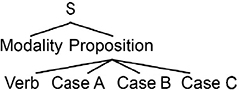
Figure 2.5. Typical structure of a sentence according to Fillmore's model
According to this approach, the modality includes information about the verbal predicate such as the time, mode, and type of sentence: affirmative, interrogative, declarative, negative, and the aspect, the representation of the locutor of the action expressed by the verb (see the example in Figure 2.5).
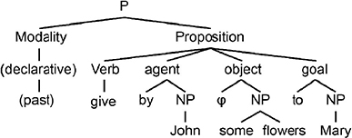
Figure 2.6. Deep structure of the sentence John gave flowers to Mary
The proposition represents the relation of the verb with one or more nominal groups in an atemporal manner (see examples in Figure 2.7).
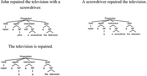
Figure 2.7. Representations of the sentence: John repaired the television with a screwdriver
During the 1970s and 1980s, Fillmore’s work on case grammar gave rise to a new theoretical framework called frame semantics. This theory combined linguistic semantics and encyclopedic knowledge. It influenced the work of Ronald Langacker on cognitive grammar [LAN 87]. Other researchers, notably including Walter Cook, John Anderson and Lachlan Mackenzie, also worked on the development and application of case grammar [COO 71, COO 89, AND 77, MAC 81].
2.1.4. Rastier’s interpretive semantics
Founded by François Rastier, a distinguished student of Greimas and Pottier, this new version of interpretive semantics was perceived by many experts as a new synthesis of structural semantics. It was developed in the wake of the works of European linguists Saussure, Hjelmslev, Greimas and Pottier [HEB 12].
Before presenting Rastier’s semantic approach, it is important to first present the levels of linguistic description that he identifies in order to clarify his terminology and situate his work within the general context:
- – The level of the morpheme: two types of morphemes are identified. Grammatical morphemes constitute a closed class in a given synchronous state. For example, the plural marker -s as in houses, the inflectional morpheme ending -ed as in walked. Lexical morphemes (lexemes) belong to one or more loosely closed classes.
- – The level of the lexia: the lexia is a group of integrated morphemes that constitute a unit of meaning. This includes simple lexia that are composed of a single morpheme and complex lexia that are composed of several morphemes. When they are written in several words, complex lexia can be classified into two groups: those that do not allow for the insertion of morphemes (maximal integration/total fixation) like in single file, and those that do allow for insertions (partial fixation) like to step up to the plate, to step up quickly to the plate [RAS 05a]. Note that, according to Rastier, the lexia is the most strongly integrated syntactic unit. Composed of one or more sememes, the signified of a lexia is a semia. It can be composed of one or more sememes.
- – The level of the syntactic unit: considered to be the true place of predication, according to Rastier, the syntactic unit is the most important for morphosyntactic constraints.
- – The level of the period: Rastier prefers to use the word period rather than the word sentence, which he considers to be a normative ideal created from the connection between grammar and logic. Notably elaborated by [CHA 86, BER 10], the period is the unit above the syntactic unit and its limits are rhetorical rather than logical. In speech, it is a respiratory unit. Generally, in speech and writing, it is a segment that can be defined using privileged local semantic relations between syntactic units (e.g. the phenomena of anaphora and coreference). The period defines the first level of a hermeneutic whole [RAS 94].
- – The level of the text: this is a higher level of complexity on which other levels depend. This level is governed by discursive and stylistic norms6. According to Rastier, the semantic structure of texts can be described using a three-tiered model: microsemantics, the level of the morpheme and lexia; mesosemantics, the level of the syntactic unit and the period; and macrosemantics, the level of units above the period all the way up to text.
Microsemantics are the semantics of the level below the text. Its upper limit is the semia (the signified of a lexia). Three sections can be distinguished in microsemantics: semes, lexicalized units and contextual relations [RAS 05a].
A sememe is a structured set of features that are deemed pertinent, called semes. There are two types of semes: generic semes and specific semes.
Generic semes are inherited from higher classes in the hierarchy (hyperonyms). They make it possible to mark relations of equivalence between the sememes. Rastier proposes distinguishing between three types of generic semes:
- – Microgeneric: semes that indicate that a sememe belongs to a taxeme. According to Rastier, the taxeme is a minimal class of sememe. For example, bus and metro belong to the taxeme of /urban transportation/ and coach and train belong to the taxeme of /inter-urban transportation/. Taxemes are a minimal class of semia. For example, /funerary monument/ for “mausoleum” and “memorial”.
- – Mesogeneric: semes that indicate that a sememe belongs to a domain. The domain is the class of the level above the taxeme. It is related to a social practice. For example, canapé can refer to the domain //house// or the domain //food//.
- – Macrogeneric: semes that indicate that a sememe belongs to a dimension. The dimension is a class of sememes or semia, of a higher level of generality, independent of domains. For example: //animate//, //inanimate//, or //human//, //animal//.
To illustrate this concept, Rastier studied the following four semias in the domain of transportation: train, metro, bus and coach. Two analyses are possible for these semias (see Table 2.1).
Table 2.1. Analyses of semias: train, metro, bus and coach
| First analysis | Second analysis | ||
|---|---|---|---|
| //transportation// | //transportation// | ||
| //rails// “metro” /intra-urban/ “train” /extra-urban/ |
//road// “bus” /intra- urban/ “coach” /extra- urban/ |
//intra-urban// “metro” /rails/ “bus” /road/ |
//inter-urban// “train” /rails/ “coach” /road/ |
Although they are semantically valid, each of these analyses is preferred in a given context: in a technical context, the first analysis tends to be preferred, whereas in daily life, the second system is used. Finally, it is important to note that the generic semes of a sememe form its classeme.
In turn, specific semes serve to oppose a sememe to one or more other sememes in the same taxeme. For example, zebra is opposed to donkey by the (specific) seme /striped/. Similarly, mausoleum is opposed to memorial by the seme /presence of a body/. The specific forms of a sememe form a semanteme.
Both of these types of semes can have two different statuses that characterize their modes of actualization: inherent semes and afferent semes.
Inherent semes make it possible to define the type. They are inherited by default if the context does not forbid it. For example, /yellow/ is an inherent seme to banana because the typical color of a banana is yellow. Although it is inherited by default, this value can be changed by a different contextual instantiation such as: Patrick painted a purple banana. Thus, no inherent seme manifests in all contexts.
There are two kinds of afferent semes: socially normed semes and contextual semes. Socially normed semes indicate paradigmatic relations that can be applied from one taxeme to another. As they do not have a defining role (unlike inherent semes), these semes are normally latent. It is therefore only possible to actualize them through a contextual instruction. If, when talking about a shark, we evoke its extraordinary capacity to catch and kill its prey, the emphasis is therefore on the seme /ferocious/. The same applies when qualifying a businessman as a shark. Because contextual semes are not proper to the lexical item, they are transmitted through determinations or predications. The specificity of these semes is that they only involve the relations between occurrences, not considering the type. For example, in the domesticated zebra, the seme /domesticated/ must be represented in the occurrence of zebra.
Three interpretive operations about semes are proposed by Rastier to account for the transformations of significations encoded in languages [RAS 05a]: activation, inhibition and propagation. Governed by the laws of dissimilation and assimilation, these operations make it possible to increase semantic contrasts.
Inhibition is an operation that consists of blocking the actualization of inherent semes. Inhibited semes are therefore virtualized. For example, the inherent feature /animal/ of the word horse is actualized in the contexts such as John rides his horse every morning. In contrast, the same feature is inhibited in nominal locutions like: Trojan horse, get off your high horse, dark horse or straight from the horse’s mouth.
Activation is an operation that allows the actualization of semes. Since inherent semes are actualized by default, activation only applies to afferent semes. For example, the seme /upright/ is not an inherent seme for the word shepherd. It is a virtual seme that can be inferred from the inherent seme /human/. In the context of O Eiffel7 Tower shepherdess, by assimilation, the seme /upright/ is actualized by the presence of the inherent seme of tower: /verticality/.
The operation of propagation concerns contextual afferent semes given that the propagation of generic features occurs more naturally than specific features, which require particular contexts like metaphors or similes. For example, the word doctor entails neither the seme /meliorative/ nor the seme /pejorative/. However, in a context such as: John is not a quack, he’s a doctor. Opposed with the word quack, which has /pejorative/ as an inherent feature, the word doctor acquires the feature /meliorative/. It is also useful to note that proper names of people lend themselves well to the propagation of semes, as their signifieds entail very few inherent semes. For example, characters in literary works represented by their proper names. Thus, Sherlock Holmes, the well-known character created by Sir Arthur Conan Doyle, only has two inherent features: /human/ and /masculine/. In the context of the novels, he receives the feature /strong observation/ and /high logical reasoning/.
As emphasized by Rastier, the interpretive operations just described are only applicable if certain conditions are met. Thus, to start an interpretive process, it is necessary to distinguish between the problem that it makes it possible to solve, the interpretant that selects the inference to be conducted, and the reception conditions that allow or facilitate the process. For example, some processes are facilitated within the same syntactic unit.
It should be noted that Rastier, based on his study of the possibilities of applications of the operations, proposes these three general principles. First, all semes can be virtualized by context. Second, only context makes it possible to determine whether a seme can be actualized or not. Third, there is no seme (inherent or not) that is actualized in all possible contexts.
Mesosemantics concerns the level between the lexia and the text. Thus, it pertains to the space that extends from the syntactic unit to the complex sentence [RAS 05b]. Although it is central in most linguistic studies, according to Rastier, syntax plays a secondary role in the domain of interpretation because he considered that ultimately, it was the hermeneutic order that took precedence over the syntagmatic order that includes syntax: semantic relations connect all sentences to their situational contexts.
Initially proposed by [GRE 66] to account for the homogeneity of discourse, the concept of isotopy is used by Rastier to illustrate relations that are deemed relative between syntax and semantics. It consists of the repetition of a seme, called an isotopizing seme, from one signified to another occupying a different position. For example, consider the text fragment [2.8]. In this fragment, the isotopy /urban transportation/ is formed by the repetition of the seme of the same name with the words taxi, driver and boulevard that possess this seme:
- The taxi is driving 100 km/h down boulevard St. Germain. [2.8]
- The driver must be crazy...
Following the status of the semes that they imply, Rastier distinguishes two types of isotopies: generic isotopies and specific isotopies.
Generic isotopies are divided into three sub-types:
- – A microgeneric isotopy is marked by the recurrence of microgeneric semes. For example, the feature /telecommunications/ in telephone and cell phone and the feature /equine/ in a sorrel horse.
- – A mesogeneric isotopy is defined as the recurrence of a mesogeneric seme. For example, the feature /writing tool/ in a pen and a pencil.
- – A macrogeneric isotopy concerns the recurrence of a macrogeneric seme. For example, the feature /animated/ in beauty and the beast.
Specific isotopies can index sememes belonging to the same domain or to the same dimension, like tiger and zebra.
As noted by Rastier, isotopies also play a fundamental role in anaphors. As these only have a small number of inherent features, most of their afferent features are naturally propagated by context. This propagation is selective and only concerns part of the features of an anaphorized unit. It consists of phenomena that also concern the mesosemantic level as much as the macrosemantic level, because many cases of anaphors can surpass the framework of the sentence or the period.
According to Rastier’s approach, the issue of relations between syntax and semantics can be reduced to relations between isosemy, prescribed by the functional system of language, and facultative isotopies, prescribed by other systems of norms [RAS 05b]. By limiting himself to facultative generic isotopies that index sememes and semias belonging to a single semantic domain, Rastier obtained these five configurations:
- – Neither facultative isotopy nor isosemy: sequences that are neither sentences nor utterances. For example: I slowly school the days mornings factory.
- – Isosemies, but not facultative isotopy: statements that are syntactically correct but for which no valid semantic interpretation exists, such as: the Manichean chair travels through illegal yellow concepts.
- – Two interlaced domain isotopies, for example: O Eiffel Tower shepherdess today your bridges are a bleating flock8 (French poet Apollinaire). The utterance creates a complex referential impression, and it is undecidable because we cannot say whether it is true or false.
- – A facultative isotopy, but with a rupture of isosemies, for example: the gun furiously searches for its bullets while aiming at the inattentive game. The words gun, bullets and game make up a seme that indexes them in the domain /hunting/. However, the world to which this utterance refers is both counterfactual and logically false.
- – A facultative isotopy and isosemies: this includes decidable utterances where several sememes are indexed in a single domain. John, a first-rate runner, won his first Olympic medal.
Thus, for interpretive semantics, the interpretability of an utterance depends more on its facultative isotopies than its obligatory isotopies. Morphosyntax has a secondary place in the domain of interpretation.
Macrosemantics concerns the level of units above the period up to the text. Rastier considered that the production and interpretation of texts was the result of the non-sequential interaction thematic, dialectic, dialogic and tactic (see Figure 2.8).
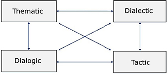
Figure 2.8. Interactions of the independent components of macrosemantics
The following paragraphs include a brief presentation of each of these components.
The thematic concerns the content of the text by specifying the topics that it addresses. According to Rastier, two types of topics can be distinguished: generic topics and specific topics.
Generic topics, or generic isotopies, are defined by a seme or a structure of generic semes. This recurrence defines an isotopy or isotopic bundle [RAS 05a]. Generic topics can take several forms such as taxemic topics, which pertain to members of the same taxeme. For example, a text that contains occurrences of cargo, boat and ship addresses the topic of //means of maritime transportation//. Similarly, there are domain topics (pertaining to members of the same domain), dimensional topics (pertaining to members of the same dimension) and semantic field topics.
Specific topics, also known as semic molecules, are recurring groups of specific semes. They can be presented in the form of a microsemantic graph without being actualized in lexical form. Rastier provides the example in Emile Zola’s novel L’Assommoir9 of a semic molecule that groups the semes /yellow/, /hot/, / viscous / and / harmful /, which are lexically realized by alcohol, sauce, mucus, oil and urine. Note that, in technical texts, semic molecules are generally lexicalized by terms.
Accounting for represented intervals of time, the dialectic is defined in two levels: the event level and the agonistic level. It allows for a dialectic typology and provides more detail about the concept of the narrative text10.
The event level has three basic units: actors, roles and functions. An actor is the aggregation of the anaphoric actants of periods (mesosemantic unit). In the period, the actants can be named or have various descriptions. Each denomination or description lexicalizes one or more of the actor’s semes. Roles are afferent semes that include the actant. They consist of semantic cases associated with the actants (accusative, ergative, dative, etc.). Functions are typical interactions between actors. They are defined by a semic molecule and generic semes. For example, the gift is an irenic function whereas the challenge is a polemic function. Each function has its own actor valence. For example, a [CHALLENGE] function can be written as: [A]<—(ERG)<—[CHALLENGE]—>(DAT)—>[B], where [A] and [B] are the actors.
Note that the semic relations between actants and functions explain the concordance or rection relations that are established between them.
Hierarchically superior to the event level, the agonistic level only appears in mythic texts and essentially only applies to technological texts. Two basic units can be identified in this level: agonists and sequences. An agonist is a type of a class of actors often indexed on different isotopies. For example, in Toine11 by Maupassant, an old woman (an actor of human isotopy), the rooster (an actor of animal isotopy), and death (an actor of metaphysical isotopy) are metaphorically compared (see [RAS 89]). Sequences are defined by the homologation of functional isomorphic syntactic units. For example, in Dom Juan12 by Molière, there are 118 functions that can be grouped into only eleven sequences (see [RAS 73]). The sequences are ordered by logical narrative relations that are not necessarily chronological.
The dialogic accounts for the modalization of semantic units at all levels of complexity of the text. It concerns aspects of texts, especially literary texts, such as the universe, worlds and narration.
This component pertains to the linear order to semantic units at all levels. Although this order is directly related to the linearity of the signifiers, it does not combine at all levels.
2.1.5. Meaning–text theory
Meaning–text theory is a functional model of language that was initially developed in the Soviet Union by [ZOL 67] and then developed at the Université de Montréal, notably by Igor MEL’CUK (see [MEL 97, MEL 98, POL 98], and for a presentation of its NLP applications, refer to [BOL 04]). This theory is based on three premises:
- – Language is a finite set of rules that establish a many-to-many correspondence between an infinite, uncountable set of meanings and an infinite, uncountable set of linguistic forms that are texts. This premise can be diagrammed like this:
- {RSemi} language;<==>; {RPhonj} | 0 < i, j ∞
where RSem is a semantic representation and RPhon is a phonetic representation of the text.
- – The input of a meaning–text model is a semantic representation and its output is the text. This correspondence must be described by a logic device that constitutes a functional model of language.
- – The logic device of the second premise is based on two intermediary levels: words and sentences. These two intermediary levels correspond to morphological and syntactic patterns, respectively.
As shown by the architecture of the meaning–text model presented in Figure 2.9, the input of this model is a semantic representation. Getting to an output that is a corresponding sentence in phonetic transcription requires going through intermediary syntactic and morphological representations.
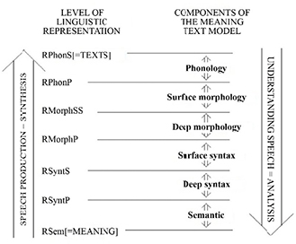
Figure 2.9. Architecture of the meaning-text model [MEL 97]
In Figure 2.9, the meaning–text model is a functional approach that describes language according to its mode of use: comprehension or production. Meaning–text correspondences are described by functions, in the mathematical sense, that establish a link between a meaning and all of the texts that express it. To describe an utterance, six levels of intermediary representation are used in addition to the levels of meaning and text. The articulation of a surface level and a deep level for the morphology and syntax serves to distinguish what is directed toward meaning from what is directed toward the text. The representations are made of formal objects called structures. The focus of this work is limited to the semantic level, which interests us the most in this context.
The semantic representation (RSem) includes three structures: the semantic structure, the semantic-communicative structure and the rhetorical structure.
The semantic structure and core of RSem corresponds to propositional meaning. It is a network whose nodes are labeled by semantic categories that are senses of the lexias of the language. The arcs of the network are labeled by numbers that specify the arguments of the predicate. To write the semantic structures, a formal language in the form of a network is used where the arcs indicate the predicate argument relations. For example, the predicate p(x, y) is represented with the network in Figure 2.10.
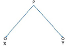
Figure 2.10. Semantic network of the predicate p(x, y) [MEL 97]
The semantic component is a set of rules that ensures correspondence with the deep level of syntactic representation (RSyntP).
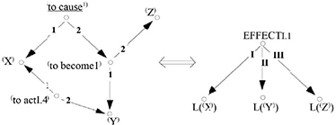
Figure 2.11. Lexical semantic rule R1 [MEL 97]
In Figure 2.11, the notation L(α) signifies that the lexia L expresses the meaning α. The rule R1 stipulates that the meaning (X, acting on Y, causes Y to become Z) can be expressed by the lexeme EFFECTI. 1: the effect Z of X on Y. It should be noted that the lexical rules are the core of entries in a new type of dictionary: the explanatory combinatorial dictionary [MEL 84].
The semantic-communicative structure expresses the oppositions between the following pairs: topic and neutral, given and new, and emphatic and neutral. Finally, the rhetorical structure concerns the locutor's intentions such as irony or pathos.
2.2. Formal semantics
The idea of using mathematics as a universal framework for human thinking goes back at least to Descartes. Mathematics has the advantage of being systematic and clear due to the absence of ambiguities, the main problem of natural languages. In the same vein, the British logician and philosopher Bertrand Russell published his book Principia Mathematica in three volumes in 1910. Written in collaboration with Alfred North Whitehead, this work developed a symbolic language designed to avoid the ambiguities of natural languages. In turn, the German–American philosopher Rudolf Carnap also contributed by developing a symbolic logic that used mathematical notation to indicate the signification of signs unambiguously. This logic is, in a way, a formal language that serves as a metalanguage designated as the semiotics of this language. In this semiotics, each sign has a truth condition. When this condition is satisfied, the meaning of a sign corresponds to what it designates.
As noted in [BAC 89], logical semantics is based on two premises. The first premise, identified by Chomsky, is that linguistics can be described as a formal system. The second premise, formulated by [MON 70], is that natural languages can be described as interpreted formal systems.
Logical semantics was not unanimously accepted by linguists. Among others, it was criticized by François Rastier, who believed that it did not treat the linguistic signified but rather related it back to a logical form [RAS 01]. However, the existence of computer languages that adopt a logical framework like Prolog makes formal approaches an attractive choice for the computational processing of meaning.
Several types of logic were used to represent meaning. This presentation will examine the two main types: propositional logic and predicate logic.
2.2.1. Propositional logic
2.2.1.1. The concept of proposition
Propositional logic concerns declarative sentences that have a unique truth value (true or false). Sentences are the smallest logical unit that cannot be further broken down (see [DOY 85, LAB 04, AMS 06, GRA 04, ALL 01, KEE 05] for more detailed introductions to propositional logic). Consider the following sentences [2.9]:
- a) Sydney is the capital of Australia. [2.9]
- b) The lowest point on earth is located near the Dead Sea.
- c) The Euphrates is the longest river in the world.
- d) John will defend his thesis on June 12th.
- e) No, thank you.
- f) One kilo of tomatoes, please.
- g) That’s not exactly true.
In the series of examples in [2.9], sentences a–d are propositions that have specific truth values even if, at a given moment, certain values are not known as in the case of d (the date of his defense can change at any time). Sentences e and f are not propositions because they are not declarative and do not have a truth value. Sentence g can have two truth values at the same time, which is why it is not a proposition.
2.2.1.2. Logical connectives
Propositions only correspond to one particular type of sentence: simple sentences. For more complex forms of sentences, specific operators called logical connectives must be used. There are five of these connectives: negation, conjunction, disjunction, implication and biconditional. These connectives act as operators on the truth values of propositions.
In propositional logic, the negation of a proposition consists of inverting its truth value. Thus, the proposition ¬P (sometimes written as ~P and read as not P) is true if P is false. Inversely, it is false if P is true. This gives us the truth table in Table 2.2.
Table 2.2. Truth table for the negation operator
| P | ¬P |
|---|---|
| T | F |
| F | T |
Note that the variable P can correspond to a simple proposition or a more complex proposition like ¬(Q ∧ R). Unlike natural languages where negation can concern several constituents, in propositional logic, negation can only pertain to the whole proposition. For example, in the sentence, John did not study at the faculty of medicine in Paris last year, the negation concerns three parts of the sentence that convey different information: study, at the faculty of medicine in Paris and last year. Sometimes, propositional negation corresponds to a total negation (that concerns the entire sentence). John is not agreeable is the equivalent of: ¬ (John is agreeable). This kind of negation can be realized with a morphological prefix: in-, im-, il- and ir-. For example, The President of the Republic is ineffective is equivalent to ¬ (The President of the Republic is effective).
Conjunction (∧) relates two propositions, P and Q, whose truth values are given in Table 2.3. It is sometimes written as (P & Q) and is read as: P and Q.
Table 2.3. Truth values for the conjunction operator
| P | Q | P ∧ Q |
|---|---|---|
| T | T | T |
| F | F | F |
| T | F | F |
| F | T | F |
Assuming that the propositions John saw the painting, John liked the painting correspond to propositions P and Q respectively, then the following sentences can be formulated logically in this way:
| a) John saw the painting and he liked it. | P ∧ Q |
| b) John saw the painting but he didn’t like it. | P ∧ ¬Q |
| c) John saw the painting. However, he didn’t like it. | P ∧ ¬Q |
| d) John liked the painting although he had not seen it. | Q ∧ ¬P |
Note that the logical equivalence between (P ∧ Q) and (Q ∧ P) is always valid. However, there are cases where this equivalence is not valid in natural language. For instance, consider the example: John opened the door and he left his house. The change in the order of propositions here implies a semantic change as the idea of coordination is paired with the idea of a chronological succession of events expressed by the propositions. With verbs that express reciprocity, like to date, to marry, to affiance and to love, the coordination in natural languages does not translate by using a logical and.
Disjunction (∨ / ∨∨) of two propositions P ∨ Q, which is read as P or Q, is true if at least one of the propositions is true. This operator is called inclusive disjunction. Its truth table is provided in Table 2.4.
Table 2.4. Truth table for the or operator
| P | Q | P ∨ Q |
|---|---|---|
| T | T | T |
| F | F | F |
| T | F | T |
| F | T | T |
Inclusive disjunction is observed in sentences like:
| John or Mary go to school. | (John goes to school) ∨ (Mary goes to school) |
| John works in the library or at home. | (John works at the library) ∨ (John works at home) |
There is a variant of disjunction called exclusive disjunction (noted as ∨∨ or XOR) that is only true if one of the two propositions is true: it is false if the two propositions are true or false. P ∨∨ Q is read as P or Q but not both. See Table 2.5 for the truth table of this variant.
Table 2.5. Truth table for the exclusive or operator
| P | Q | P ∨∨ Q |
|---|---|---|
| T | T | F |
| F | F | F |
| T | F | T |
| F | T | T |
In daily life, the exclusive or designates an action that only takes a single agent as in John or Michael is driving Mary’s car. This also translates into expressions such as Either John or Mary is leaving on a mission to Paris.
Implication is represented by the operator →. If P and Q are propositions, then P → Q, is read as: if P then Q or P implies Q, is a proposition whose truth table is provided in Table 2.6.
Table 2.6. Truth table for the implication operator
| P | Q | P → Q | |
|---|---|---|---|
| 1 | T | T | T |
| 2 | F | F | T |
| 3 | F | T | T |
| 4 | T | F | F |
In Table 2.6, P → Q is false only if P is true and Q is false. To clarify this table, consider the four sentences below, which correspond to the four lines in the truth table, respectively:
- 1) If it is nice out, I will go play sports in the park.
- 2) If London is the capital of the Maldives, then Paris is the capital of Sri Lanka.
- 3) If you are Marie Antoinette’s friend, then the Earth is round.
- 4) If Damascus is the capital of Syria, then 8 + 5 = 20.
Propositions 2 and 3 indicate that anything can be deduced from something that is false. Proposition 4 is false because something false cannot be deduced from something that is true. Note that more complex propositions can be part of an implication as in this sentence: if it is nice out (P) and if I am not tired (¬Q), then I will go play sports (R).
The biconditional, represented by the operator ↔, expresses a relation of equivalence between two propositions. The proposition P ↔ Q (which is read as P if and only if Q) is true if the two propositions P and Q have the same truth. This results in the truth table provided in Table 2.7.
Table 2.7. Truth table for the biconditional
| P | Q | P↔Q |
|---|---|---|
| T | T | T |
| F | F | T |
| T | F | F |
| F | T | F |
From a logical perspective, P↔Q is equivalent to P → Q ∧ Q → P. Expressed in English, this relation is translated by expressions such as: only if, without which, unless. Consider the following sentences and their implications:
| I will come to the game (p) unless I am on a trip. (Q). | P↔Q |
| If I am on a trip, then I will not come to the game. | Q → P |
| If I come to the game, then I am not on a trip. | P → Q |
2.2.1.3. Well-formed formulas
A well-formed formula (wff) is a logical expression that has a meaning. A simple variable that represents a proposition P is the simplest form of a wff. Connectives can be used to obtain more complex wffs. For example: (¬P), (p ⋀ ¬Q), (¬¬P), etc. More formally, a wff can be defined according to these criteria:
- i) All atomic propositions are wffs.
- ii) If P is a wff, then ¬P is a wff.
- iii) If P and Q are wffs, then (P ∧ Q), (P ∨ Q), (P → Q), (P ↔ Q) are wffs.
- iv) A sequence is a wff if and only if it can be obtained by a finite number of applications of (i)–(iii).
By replacing the variables of a wff α with equivalent propositions, the truth value of this formula can be calculated from the truth values of the propositions that compose it. Consider this formula and its truth table presented in Table 2.8:
Table 2.8. Truth table for formula α
| P | Q | (P ∨ Q) | (P → Q) | (P → Q) ∧ (Q → P) | (Q → P) | α |
|---|---|---|---|---|---|---|
| T | T | T | T | T | T | T |
| T | F | T | F | F | T | F |
| F | T | T | T | T | F | F |
| F | F | F | T | F | T | F |
Note that the number of lines in the formula increases with the number of variables in the formula. It is equal to 2n, where n is the number of variables in the formula. This means that the number of lines in the truth table of a formula with two variables is equal to four, and for a formula with three variables, there are eight lines, and so on.
Some formulas have the truth value T, regardless of the value of the propositions that compose them. In other words, they are always true. This type of formula is called a tautology. The formulas P ∨ ¬P, (P ∧ Q) ∨ ¬P ∨ ¬Q are examples of tautologies. Another particular case of a wff is absurdity or contradiction. This is a wff that, unlike a tautology, has the truth value F, regardless of the truth value of the propositions that compose it. For example, P ∧ ¬P, (P ∧ Q) ∧ ¬Q. Because absurdity is the opposite of a tautology, α is an absurdity if ¬α is a tautology, and vice versa.
Two wffs α and β with propositional variables p1, p2, …., pn, etc. are logically equivalent if the formula α ↔ β is a tautology. Therefore, this is written as α ≡ β. This means that the truth tables of α and β are identical. For example:
P ∧ P ≡ P, consider the truth table for the two formulas presented in Table 2.9.
Table 2.9. Proof of P ⋀ P ≡ P
| P | P ∧ P |
|---|---|
| T | T |
| F | F |
Because the columns corresponding to the formulas are identical, this proves that the formulas are equivalent. To prove the equivalence: P ∧ Q ≡ Q ∧ P, consider the truth table for the two formulas presented in Table 2.10.
Table 2.10. Proof of P ⋀ Q ≡ Q ⋀P
| P | Q | P ∧ Q | Q ∧ P |
|---|---|---|---|
| T | T | T | T |
| T | F | F | F |
| F | T | F | F |
| F | F | F | F |
To clarify the concept of proof of equivalence, consider one final example, (p → (Q ∨ R)) ≡ ((P → Q) ∨ (P → R)) whose equivalence is proven in Table 2.11 where the two wffs have exactly the same truth values.
Table 2.11. Proof of (p → (Q ∨ R)) ≡ ((P → Q) ∨ (P → R))
| P | Q | R | Q ∨ R | p → (Q ∨ R) | P → Q | P → R | (P → Q) ∨ (P → R) |
|---|---|---|---|---|---|---|---|
| T | T | T | T | T | T | T | T |
| T | T | F | T | T | T | F | T |
| T | F | T | T | T | F | T | T |
| T | F | F | F | F | F | F | F |
| F | T | T | T | T | T | T | T |
| F | T | F | T | T | T | T | T |
| F | F | T | T | T | T | T | T |
| F | F | F | F | T | T | T | T |
It should be added that there are particular equivalencies that serve to deduce other equivalencies by simplifying the formulas. These are called identities. If a formula β is part of a formula α and if β is equivalent to β’, then it can be replaced with β’ and the formula obtained is a wff equivalent to α. Figure 2.12 provides a few examples of logical identities commonly used in deductions.
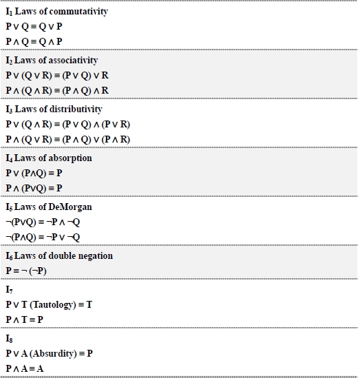
Figure 2.12. A few logical identities
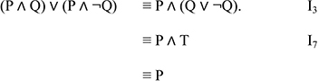
To illustrate the use of these rules in the proof process, consider the following example: (P ∧ Q) ∨ (P ∧ ¬Q) ≡ P. The proof consists of simplifying the left side until P is obtained.
2.2.1.4. Rules of inference
Rules of inference are tautologies that have this construction: ![]()
They are similar to an implication: Premises → Conclusion. The part that concerns the premises pertains to the proposition that is assumed to be true. It is sometimes called the hypothesis. The conclusion concerns the proposition derived from the premises. The valid process argument concerns arriving at the conclusion from the premises. Some deduction rules and their equivalents in the form of inferences are given in Figure 2.13.
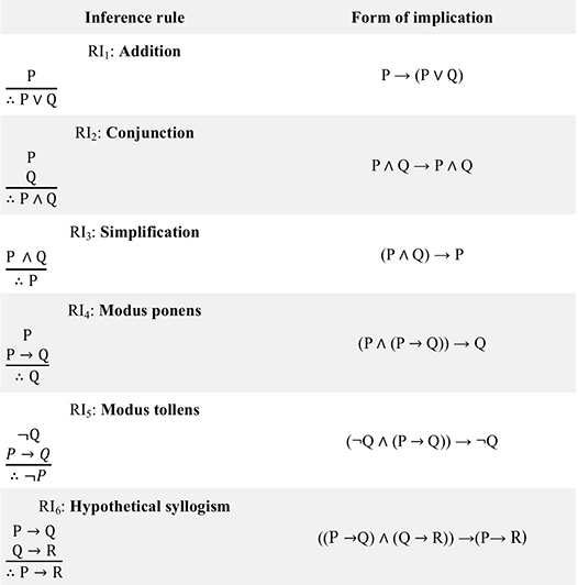
Figure 2.13. A few rules of inference
Consider the following argument:
If John won an Olympic medal or if he won a gold medal at the world championships, then he is certain to receive the Legion of Honor13. If John is certain to receive the Legion of Honor, then he is happy. Or, he is not happy. Then, he did not win a gold medal at the world championships.
To verify the validity of such an argument, follow these steps.
- 1) Identify the propositions:
- – P signifies: John won an Olympic medal.
- – Q signifies: John won a gold medal at the world championships.
- – R signifies: John is certain to receive the Legion of Honor.
- – S signifies: John is happy.
- 2) Determine the left and right sides of the rule of inference:
The premises of the inference are:
- i) (P ∨ Q) → R
- ii) R → S
- iii) ¬S
The conclusion is: ¬Q
i) (P ∨ Q) → R Premise (i) ii) R → S Premise (ii) iii) (P ∨ Q) → S Hypothetical syllogism RI6 iv) ¬S Premise (iii) v) ¬(P ∨ Q) Modus tollens RI5, lines 3 and 4. vi) ¬P ∧ ¬Q Law of DeMorgan vii) ¬Q Simplification RI3 - 3) It can be concluded that the argument is valid.
In short, propositional logic is a declarative system that makes it possible to express partial knowledge, disjunctions, negatives, etc. However, contrary to natural languages, in propositional logic, meaning is independent of the context. Thus, each fact to be represented requires a separate proposition. This means that the representation process is not very efficient and sometimes insufficient. Propositional logic is incapable of adequately processing the properties of individual entities such as the Mona Lisa and Picasso or their relations to other entities. In addition, cases like [2.10] present difficulties for the logic of propositions because they require a mechanism that is not available in this type of logic. This concerns quantifiers that are available in the upper level logics like first-order logic:
- – Everyone likes nature. [2.10]
- – There is always someone to love a child.
2.2.2. First-order logic
First-order logic makes it possible to represent the semantics of natural languages in a more flexible and compact way than propositional logic. Contrary to the logic of propositions, which assumes that the world only contains facts, this logic assumes that the world contains terms, predicates and quantifiers.
2.2.2.1. Terms
To refer to individuals, first-order logic uses terms. These are specific objects that can be constant, like 10, Paul, and Lyon, or variables such as X, Y, Z. The functions of the form f(t1,...,tn) are terms whose parameters ti are also terms. For example, the function prec(X) is a function that takes an integer and gives the arithmetically preceding integer (prec(X) = X−1). Another example of a function with several parameters is addition +(X, Y)=X + Y.
2.2.2.2. Predicates
Predicates are used to describe terms or to express the relations that exist between them. This is how predicate logic expresses propositions. Generally, unary predicates, with a single argument, can represent the properties or simple actions that can be true or false. For example: intelligent (John), left (John) and carnivore (tiger). N-ary predicates, with n arguments where n is greater than 1, represent predicates with several arguments. For example: the predicate mother (Mary, Theresa) can be used to designate Mary as the mother of Theresa or the inverse, with order being a question of convention. Similarly, the predicate: to leave (John, Cleveland, Chicago) can be interpreted as: John left from Cleveland for Chicago or from Chicago for Cleveland. Connectives can be used to express more complex facts, as in the sentences in [2.11] and their representations in first-order logic:
- Theresa is the mother of John and Mary. [2.11]
- mother(Mary, Theresa) Λ mother(John, Theresa).
- John likes oranges but he doesn’t like apples.
- like(John, Orange) ∧ ¬like(John, apple).
- Mary is studying pharmacy or medicine.
- study(Mary, pharmacy) ∨ study(Mary, medicine).
2.2.2.3. Quantifiers
Quantifiers make it possible to express facts that apply to a set of objects, expressed in the form of terms, rather than on individual objects. To do the same thing in predicate logic, all of the cases must be listed, which is often impossible. For example, the sentences in group [2.12] require a representation with quantifiers:
- – Everyone loves apple pie. [2.12]
- – Everyone is at least as poor as John.
- – Someone is far from home.
Predicate logic has two quantifiers to express this kind of sentence: the universal quantifier and the existential qualifier.
The universal quantifier has the form: x p(x). It is read as for all X p(x) and signifies that the sentence is always true for all values of the variable x. Consider examples [2.13]:
| ∀x likes(x, Venice) | Everyone likes Venice. [2.13] |
| ∀x [horse(x)→ mammal(x) Λ mammal(x) →animal(x)] | Horses are mammals which are animals. |
| ∀x inherit(John, x) → book (x) | All that John inherited was a book. |
| ∀x book(x) → inherit(John, x) | John inherited all of the books (in the universe). |
The universal quantifier is often used with implication. If not, it becomes very restricting. Consider this example: ∀x apple(x) ∧ red(x). This formula translates in natural language as: everything in the universe is a red apple.
The existential quantifier is expressed in the form ∃x p(x) and is read as: there exists one x such as p(x) or there is at least one x such as p(x) and signifies that there is at least one value of x for which the predicate p(x) is true.
| ∃x bird(x) Λ in(forest, x) | There is at least one bird in the forest. |
| ∃x mother(Mary, x) Λ mother(John, x) | John and Mary are siblings. |
| ∃x person(x) Λ likes(x, salad) | There is (at least) one person who likes salad. |
| ∃x (∀y animal(y) → ¬to like(x, y)) | There is someone who does not like animals. |
| ∃x ∀y like (y, x) Λ ¬∃x ∀y like (x, y) | Everyone likes someone and no one likes everyone. |
| ∀x(∃y(mother(y, x)) Λ ∃z(y = father(z, x))) | Everyone has a father and a mother. |
From a syntactic perspective, the negation connectives and the quantifiers have the highest priority. Then come the connectives of conjunction and disjunction. After that, implication, and finally, the biconditional has the lowest priority.
| ∀x cat(X) → nice(X). | All cats are nice. |
| ∃x cat(X) Λ nice(X). | There is at least one cat that is nice. |
Note that the same thing can be expressed with the existential quantifier and the universal quantifier. Consider these basic cases:
| ∀x ¬P ↔ ¬∃x P | |
| ∀x ¬ like(x, John) ↔ ¬∃x like(x, John) | Nobody likes John. |
| ¬∀x P ↔ ∃x ¬P | |
| ¬∀x like(x, John) ↔ ∃x ¬ like (x, John) | There is at least one person who does not like John. |
| ∀x P ↔ ¬∃x ¬P | |
| ∀x like(x, John) ↔ ¬ ∃x ¬ like(x, John) | Everyone likes John. |
| ∃x P ↔ ¬∀x ¬P | |
| ∃x like(x, John) ↔ ¬∀x ¬ like(x, John) | There is at least one person who likes John. |
There are some equivalencies that allow for making simplifications. For example:
- ∀x P(x) ∧ Q(x) ↔ ∀xP(x) ∧ ∀xQ(x)
- ∃x P(x) ∨ Q(x) ↔ ∃xP(x) ∨ ∃xQ(x)
To talk about a unique case or a particular entity that performs a given action or that has a given property, as in only John makes/eats/sleeps, the following formula can be used:
∃x P(x) ∧ ∀y P(y) → (x = y). A particular version of the existential quantifier makes it possible to simplify the previous formula: ∃!x P(x).
The use of a quantifier leads to the distinction between two types of variables: bound variables, which are found in the field of a quantifier, and free variables, which are independent from quantifiers. Sometimes, in the same formula, a variable can have both free and bound occurrences. Consider the following examples to clarify the difference between bound and free variables:
- –∃x like (x, y) x is a bound variable, whereas y is a free variable.
- –∀x∃y(O(x, y)) ∨ ∃z(P(z, x)) the first occurrence of x is bound and the second occurrence is free. The variables y and z are bound.
The field of a variable makes it possible to describe some ambiguities. Consider the following sentence with its two possible paraphrases: each person (everyone) likes someone:
- – Each person has someone that they like.
- – There is a person that is liked by everyone.
The first interpretation implies a relation between two groups: several to several. On the contrary, the second interpretation of the sentence is a relation between a group and an individual: one to many. Translated logically, this provides the following formulas:
- ∀x∃y like(x, y).
- ∃x∀y like(y, x).
2.2.2.4. Well-formed formulas (wffs)
In first-order logic, the formulas are formally defined in this way:
- i) The symbols of the predicate: if P(a1, …, an) is a symbol of the predicate n-ary and t1, ..., tn are the terms, the P(t1, ..., tn) is a formula.
- ii) Equality: if the equality symbol is considered to be part of the logic and t1 and t2 as being terms, then t1 = t2 is a formula.
- iii) Negation: if φ is a formula, then ¬ φ is also a formula.
- iv) Connectives: if φ and ψ are formulas, then: (φ Λψ), (φ∨ψ), (φ → ψ), (φ ↔ ψ) are formulas.
- v) Quantifiers: if φ is a formula, then ∀x φ and ∃x φ are formulas.
- vi) Only the expressions obtained following a finite number of applications of (i)–(v) are formulas.
The formulas obtained with (i) and (ii) are called atomic formulas. For example, like(John, school) is an atomic formula whereas: go(John, school) → work(John) ∨ play(John) is a complex formula. The formulas can be analyzed in the form of trees made up of the atomic formulas that constitute them. Consider the following formula p → (q ∨ r), analyzed in tree form as in Figure 2.14.

Figure 2.14. Tree structure of a simple formula
Consider another more elaborate example whose analysis is provided in Figure 2.15: [(p ∧ q) → (¬p ∨ ¬¬q)] ∨ (q → ¬p).
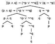
Figure 2.15. Tree structure of a more complex formula
Finally, it is useful to add that the formula, all of whose variables are bound, is called a closed formula or sentence whereas a formula with open variables is called a propositional function.
2.2.2.5. Semantic interpretation
Translating natural language sentences into a first-order logic equivalent is definitely a necessary step to reach a semantic representation of these sentences, but it is not sufficient. The logical representation must be connected to the context to express meaning. In principle, calculating the truth value of a sentence comes down to affirming or not whether it corresponds to the reality it describes. The truth value is positive or true (V = 1) in case of correspondence and negative or false (V=0) in case of non-correspondence. More formally, if the variable S is used to designate the situation described by the sentence, the sentence P is true in a situation S if [p]v=1. Where [p]v is the truth value of the sentence P. Inversely, a sentence P is false in a situation S if [p]v=0. The problem is that a sentence in natural language is composed of a set of elements such as the verb, subject nominal group, object complements, etc. To calculate the compositional meaning, the following steps are necessary:
- i) Interpreting the first-order logic symbols: unlike in proposition logic, not everything in first-order logic is a proposition. Calculating the truth value of a sentence must begin by processing the basic symbols, each of which has an interpretation. The language of first-order logic is composed of the vocabulary V that is a set of constants, functions and predicates of this language.
- ii) Defining the universe: sometimes called the domain, the universe is a representation of individuals and their relations in a given situation S. Consider, for example, the situation of the competition between David Douillet and Shinichi Shinohara for the Olympic medal in Judo in the +100 kg category in Sydney in 2000. To simplify it, the following individuals are in this situation: the two judokas, the judge and two spectators named Guillaume and Tadahiro. This gives a situation S with a set of individuals U={David, Shinichi, judge, Guillaume, Tadahiro}.
- iii) An interpretation function: the role of this function is to establish a link between the logical representations and the extensions that correspond to these representations in the situation. In our situation S, the interpretation function F(x) can give the entity denoted by x in the situation S. For example:
F(d) = David F(s) = Shinichi F(g) = Guillaume F(t) = Tadahiro F(j) = judge This function also provides the extensions of the predicates.
F(C) = combat in the Judo finals at the Sydney Olympics = {David, Shinichi} F(M) = gold medal winner in Judo at the Sydney Olympics = {David} F(A) = adjudicated the Judo finals at the Sydney Olympics = {referee} F(S) = spectators at the Judo finals at the Sydney Olympics = {Guillaume, Tadahiro} - iv) The model: this is a combination of the domain and the interpretation function. From a formal perspective, this can be represented as: Mn = (Un, Fn) where M is the model, U is the set of individuals and F is the interpretation function. The specifiers make it possible to differentiate between the situations: M1 = (U1, F1); M2 = (U2, F2), etc.
- v) Evaluating the truth values of the formulas: after having defined the general framework that makes it possible to anchor a formula in a given situation, it is necessary to define the rules (algorithms) that make it possible to decide if a formula is true or not in a given situation. Consider a simple expression like: S(ch).
In relation to the situation S, this expression signifies that Charles is a spectator at the +100 kg Judo finals at the Sydney Olympics. Intuitively, Charles is a spectator at this competition if the extension of Charles is part of the set of spectators defined by the predicate S (spectator) in the model M1. The formula to evaluate if this expression is true or not is:
- [S(c)] M1 =1 iff14 [c] M1 ∈[S] M1.
Because Charles does not belong to the set of spectators {Guillaume, Tadahiro}, then the expression S(ch) is false and its truth value is consequently equal to zero.
By taking the truth values of simple expressions as a base and considering a model M as a reference, the truth values of complex formulas can be calculated according to these rules:
- – Identity: if φ expresses an identity: α = β, then φ is true in M iff β and α correspond to the same objects in M.
- – Negation: if φ = ¬ψ, then φ is true in M, then ψ in M is false and vice versa.
- – Equality: if φ = ψ, then φ is true if φ and ψ have exactly the same truth value in M.
- – Conjunction: if φ = (α ∧ β), then φ is true in M iff α and β are true in M.
- – Disjunction: if φ = (α ∨ β), then φ is true in M iff α or β are true in M.
- – Implication: if φ = (α → β), then φ is false iff α is true and β is false.
- – Biconditional: if φ = (α ↔ β), then φ is true in M iff α and β have the same truth value in M (both are true or both are false).
- – Existential quantifier: if φ is in the form ∃x P(x), then its truth value will be true if there is u ∈U such as P(x) is true when x has the value u. In other words, φ is true if there is at least one value of x that is part of: [x] M1 ∈ [P] M1. Returning to our model, M1, the formula ∃x S(x) is true if x is equal to Guillaume or Tadahiro.
- – Universal quantifier: if φ is in the form ∀x P(x), then it is true if x takes all of the possible values in U: ∀u ∈U, x=u.
2.2.3. Lambda calculus
Lambda calculus was invented in 1936 by Alonzo Church [CHU 40], at the same time that Alan Turing invented his machine. These two formalisms have the same power of representation concerning computational calculations. Lambda calculus is a formalism just like predicate logic and first-order logic. In the domain of formal semantics, it is often considered to be an extension of first-order logic to include the operator lambda (λ) that makes it possible to connect variables. Although it initially lacked types, lambda calculus was quickly equipped with them. The types refer to objects of a syntactic nature. The non-typed variant is the simplest lambda calculus form where there is only one type. As noted in several books and tutorials entirely or partially dedicated to the subject, the use of lambda calculus became common in the domain of computational linguistics as well as in the domain of functional programming with languages like Lisp, Haskell and Python (for an introduction to lambda calculus, see [ROJ 98, MIC 89, BUR 04, BLA 05, LEC 06]). Due to its capacity to represent any computational calculation, lambda calculus lends itself well to the abstract modeling of algorithms [KLU 05].
2.2.3.1. The syntax of lambda expressions
The expression is the central unit of lambda calculus. A variable is an identifier that can be noted with any letter a, b, c, etc. An expression can be recursively defined like this:
- <expression> := <variable> | <function>|<application>
- <function> := λ<variable>.<expression>
- <application> := <expression><expression>
The only symbols used by the expressions are the λ and a period. This gives expressions like:
| λx.x | Identity function. |
| (λx.x)y | Application of a function to an expression. |
| λx.large(x) | An expression with a variable. |
| λxλy.eat(x)(y) | An expression with two variables. |
The expression can be enclosed by parentheses to facilitate reading without affecting the meaning of this expression. If E is an expression, then the expression (E) is totally identical. That being said, there are different equivalent notations in the literature, where a period cannot be used, or in which square brackets are used to mark the extent of the lambda term. Consider the example of the predicate eat to illustrate these notations:
- λxλy[eat(x)(y)]
- λxλy(eat(x)(y))
- λxy. eat(x)(y)
The applications of functions are evaluated by replacing the value of the argument x in the definition of the function: (λx.x)y = [y/x]x = y. In this transformation, [y/x] signifies that all of the occurrences of x are being replaced by y in the expression on the right. In this example, the identity function has just been applied to the variable y.
In lambda calculus, the variables are considered to be local in the definitions. In the function λx.x, the variable x is a bound variable because it is preceded by λx in the definition. On the other hand, a variable that is not preceded by λ is said to be a free variable. In the expression, λx.xy x is a bound variable while y is a free variable. A term that does not have a free variable is said to be closed or combinatory. More formally, a variable is free in these cases:
- – <variable> is free in <variable>
- – <variable> is free in λ<variable1>.<expression> if <variable> ≠<variable1> and if <variable> is a free variable in <expression>.
- – <variable> is free in E1E2 if it is free in E1 or E2.
Similarly, a variable is said to be bound in these cases:
- – <variable> is bound in λ<variable1>.<expression> if <variable> = <variable1> or if <variable> is a bound variable in <expression>.
- – <variable> is bound in E1E2 if <variable> is bound in E1 or E2.
Note that sometimes, in the same expression, a variable can be both free and bound. For example, in the expression (λx.xy)(λy.yz), the first variable y is free in the first sub-expression (on the left) and it is bound in the second sub-expression (on the right).
2.2.3.2. Types
The use of the typed version of lambda calculus offers the advantage of avoiding paradoxes and keeping the function definition within the boundaries of the standard theory of sets. Without types, we could construct terms like: the set of all sets that are not self-included. This seemingly simple expression leads to a paradox known as the Russell Paradox. If this set is not a member of itself, then it is not the set of all sets and if it is a member of itself, then it was self-included.
According to the theory of types introduced into semantics by [MON 73], a type domain for a language L is defined by two elements e and v where e corresponds to an entity and v corresponds to a truth value (0 or 1). The derived types are defined in this way:
- – e is a semantic type.
- – v is a semantic type.
- – For either of the semantic types δ, ε, < δ, ε > is a semantic type.
- – Nothing else is a semantic type.
The domains are defined in the following way:
- – De is the domain of entities or individuals.
- – Dt = {0, 1} is the domain of truth values.
- – For either of the semantic types δ, ε, D< δ, ε > is the domain of functions Dδ to Dε.
According to this definition, the sentences (propositions) are type v, the nouns are type e. The other types are constructed based on these two types. Thus, intransitive verbs and adjectives, represented by predicates with a single argument, are associated with functions of the type <e, t> because this is the function of an entity toward a truth value: e → t. Transitive verbs and prepositions (represented by predicates with two arguments) are interpreted as functions of the type: <e,<e, t>>, because it consists of a function of an entity toward a function. Finally, nominal, verbal and adjectival groups are of the type <e, t>. Their domains can be divided into subsets of various types depending on the case: Dt, De, D<e, t>, etc. Here is an example of a typed lambda formula: λP<e t>λxeP(x).
Because indicating types weigh the terms down, they are often assumed without being given explicitly.
2.2.3.3. The semantics of lambda expressions
Lambda expressions can often be interpreted in two different ways:
- a) λα[φ] the smallest function that connects α and φ.
- b) λα[φ] the function that associates α with 1 if φ, or with 0 otherwise.
Interpretation a is used when φ does not have a truth value and interpretation b is used in the opposite case. When φ is associated with a truth value, then λα[φ] is a characteristic function of a set. Therefore, lambda expressions can be considered to be a notational equivalent of sets as in the example:
This is a function that attributes the truth value 1 to x if the predicate to run (x) is true and 0 if the predicate is false.
2.2.3.4. Conversions
There are three rules that make it possible to convert or reduce the lambda expressions, two of which are relevant for this presentation: α-conversions and β-conversions.
Lambda expressions that differ only in names of variables are freely interchangeable. In other words, α-conversion stipulates that the names of variables have no importance in the expressions. The following expressions are therefore totally identical:
- (λx.x) ≡ (λy.y) ≡ (λz.z)
- (λxλy.F(x)(y)) ≡ (λzλx.F(z)(x)) ≡ (λwλz.F(w)(z))
These expressions are sometimes called α-equivalents.
β-conversion (β-reduction) is used to represent the meaning of the components of the propositions. The lambda expressions are converted by this operation to obtain a representation of the entire proposition in first-order logic, which can be used by theorem-proving algorithms. The application of the β-conversion to a formula like: λx.P(x)@(a) consists of replacing all of the occurrences of x by a which gives: P(a). Consider the following examples:
- – λx.eats (Paul, x)@(apple) → eats(Paul, apple)
- – λxλy.searches(x, y)@(John)(Mary)15 → searches(John, Mary)
- – λx.strong(x) Λ intelligent(x)@(John) → strong(John) Λ intelligent(John)
This operation also applies to predicates that make it possible to define relations as in these two examples:
- – λP.P(a)@(Q) → Q(a)
- – λyλz. want(y, z)@(John)(λx. travel(x)) → want(John, λx.to travel(x))
2.2.3.5. The use of lambda calculus in natural language analysis
According to the principle of compositionality, the meaning of an utterance depends on the meaning of its components as well as its syntactic structure. Certain semantic approaches, like that of Montague, advocate for the direct matching between syntax and semantics by associating a semantic rule with each syntactic rule. The semantic representation of basic syntactic categories will be examined first, followed by the representation of two complete sentences.
Proper nouns are type e. Some consider proper nouns to be sets of properties, a set of sets, and attribute them the type: (e → t) → t. The lambda expression corresponding to a proper noun like John is: λP.P@(John). Common nouns like girl, village and chair are considered to be properties or sets and therefore of the type (e → t). Typically, the lambda expression corresponding to a common noun like shark is in the form: λx.shark(x) expressed as the property of x such as x is a shark.
Determinants apply to common nouns and convey the higher level structure of the nominal group. Processing determinants occurs in combination with universal and existential quantifiers as in the following cases:
- – A/An: to represent this determinant, we can use the expression: λQ.∃x(P(x) ∧ Q(x)). In this expression, the capital Q is a complex variable. It marks the place of complex information that is missing from the current stage of the processing. Some researchers prefer to note these variables with the operator @, as in: λP.∃x(P(x) ∧ Q@x. Processing a nominal group like a house occurs according to the tree in Figure 2.16.
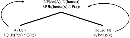
Figure 2.16 Representation of a nominal group with the determinant a
Complex variables also play a fundamental role in the representation of the other determinants:
- – Each/All: the corresponding lambda expression is in the form: λP.λQ.∀x(P(x) → Q(x)).
- – For example, all the students: λP.∀x(student(x) → P(x)).
- – Some: the lambda expression of this quantifier is: λPλQ.∃x(P(x) ⋀ Q(x)).
- – For example, some journalists: λP.∃x(journalist(x) ⋀ P(x)).
- – None or no: this uses the expression: λPλQ.¬∃x(P(x) ⋀ Q(x)).
- – For example, no children: λR¬∃x(child(x) ⋀ P(x)).
There are two opposing perspectives regarding the type of the adjective (see [TRU 04] for a more detailed discussion). On the one hand, some believe that the adjective denotes properties of the type (e, t). As shown in [PAR 87, ZAM 00], in constructions like [2.14] where an adjective can be coordinated with an indefinite determinative phrase, the adjective has a similar status:
- I consider the president intelligent and an authority in his country. [2.14]
- Je considère le président intelligent et une autorité dans son pays.
On the other hand, the standard perspective of categorial grammar that is defended by [LEW 70, KAM 75] among others considers that the adjective has an attributive nature and therefore plays the role of a predicate or a functor that takes a nominal element as an argument. This nominal element being of the type (e, t), they conclude that the type of adjective must be ((e, t) → (e, t)). Thus, the representation of an adjective like green becomes: λPx.(P(x) ⋀ green(x)).
Cases where an adjective does not modify a noun, as in [2.15], are worth mentioning. According to [KAM 75], these cases can be processed by using an implicit hyperonym. Thus, sentence [2.15] becomes Michael is a smart /boy/man/etc.
Michael is a smart. [2.15]
Verbs play the role of a logical predicate and can take zero or several arguments depending on whether they are transitive or not. The case of intransitive verbs is the simplest: they are type (e → t) and are associated with expressions like: λx.V(x). For example, the verb to run is associated with the expression: λx.to run(x). Processing transitive verbs logically is more complex. A naive solution for the processing could consist of using formulas like the one for the verb to eat: λxλy. eat(x, y). This simplistic solution is obviously not correct, given that the object of the verb is none other than a nominal group, which is in turn a structure composed of a predicate with its arguments. Therefore, the expression for a verb like to eat is: λXλz.(X@λx.eat(z, x)).
To illustrate the use of lambda calculus in the analysis process, consider a simple phrase without a quantifier such as: John looks at a flower. Analyzed syntactically, it provides the dependency tree given in Figure 2.17.
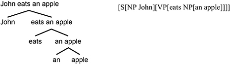
Figure 2.17. The syntactic dependencies of the sentence: John looks at a flower
The semantic relations needed are:
| John | λP.P@(John) |
| eats | λXλz.(X@λx.eat(z, x)) |
| apple | λx.apple(x) |
| An | λP. ∃x(Q(x) ∧ P(x)) |
The analysis is obtained by a successive application of β-reductions (provided in Figure 2.18).

Figure 2.18. Analysis of a simple sentence with a transitive verb
2.2.4. Other types of logic
The name “first-order logic” suggests that there are higher level logics. One of the specificities of first-order logic compared to predicate logic is to allow quantification on objects. Higher level logics allow quantification not only on objects but also on properties or relations (predicates). For example, second-order logic allows quantification on predicates and functions as in the following case:
This formula means that if x and y are equal, then they must be the same color. Third-order logic, in turn, makes it possible to quantify on the predicates of predicates, among others.
Intended for the formalization of modal information, so-called modal logic has various forms, including classic modal logic, epistemic logic (regarding knowledge), deontic logic (moral), temporal logics, etc. As an example, classic modal logic has four modalities: necessary, contingent, possible and impossible (see [BLA 01] for a formal introduction). This logic is particularly useful for modeling both human–human and human–machine dialogues [CAE 95, VIL 04].
Dynamic logics show how the representation of propositions evolves with the introduction of new information during the discourse.