Chapter 2. Question Answering
Whether you’re a researcher, analyst, or data scientist, chances are that you’ve needed to wade through oceans of documents to find the information you’re looking for. To make matters worse, you’re constantly reminded by Google and Bing that there exist better ways to search! For instance, if we search for “When did Marie Curie win her first Nobel Prize?” on Google, we immediately get the correct answer of “1903” as illustrated in Figure 2-1.

Figure 2-1. A Google search query and corresponding answer snippet.
In this example, Google first retrieved around 319,000 documents that were relevant to the query, and then performed an additional processing step to extract the answer snippet with the corresponding passage and web page. It is not hard to see why these answer snippets are useful. For example, if we search for a trickier question like “Which country has the most COVID-19 cases?”, Google doesn’t provide an answer and instead we have to click on one of the web pages returned by the search engine to find it ourselves.1
The general approach behind this technology is called question answering (QA). There are many flavors of QA, but the most common one is extractive QA which involves questions whose answer can be identified as a span of text in a document, where the document might be a web page, legal contract, or news article. The two-stage process of first retrieving relevant documents and then extracting answers from them is also the basis for many modern QA systems, including semantic search engines, intelligent assistants, and automated information extractors. In this chapter, we’ll apply this process to tackle a common problem facing e-commerce websites: helping consumers answer specific queries to evaluate a product. We’ll see that customer reviews can be used as a rich and challenging source of information for QA, and along the way we’ll learn how transformers act as powerful reading comprehension models that can extract meaning from text. Let’s begin by fleshing out the use case.
Note
This chapter focuses on extractive QA, but other forms of QA may be more suitable for your use case. For example, community QA involves gathering question-answer pairs that are generated by users on forums like Stack Overflow, and then using semantic similarity search to find the closest matching answer to a new question. Remarkably, it is also possible to do QA over tables, and transformer models like TAPAS can even perform aggregations to produce the final answer! There is also long form QA, which aims to generate complex paragraph-length answers to open-ended questions like “Why is the sky blue?”. You can find an interactive demo of long form QA on the Hugging Face website.
Building a Review-Based QA System
If you’ve ever purchased a product online, you probably relied on customer reviews to help inform your decision. These reviews can often help answer specific questions like “does this guitar come with a strap?” or “can I use this camera at night?” that may be hard to answer from the product description alone. However, popular products can have hundreds to thousands of reviews so it can be a major drag to find one that is relevant. One alternative is to post your question on the community QA platforms provided by websites like Amazon, but it usually takes days to get an answer (if at all). Wouldn’t it be nice if we could get an immediate answer like the Google example from Figure 2-1? Let’s see if we can do this using transformers!
The Dataset
To build our QA system, we’ll use the SubjQA dataset2 which consists of more than 10,000 customer reviews in English about products and services in six domains: TripAdvisor, Restaurants, Movies, Books, Electronics, and Grocery. As illustrated in Figure 2-2, each review is associated with a question that can be answered using one or more sentences from the review.3
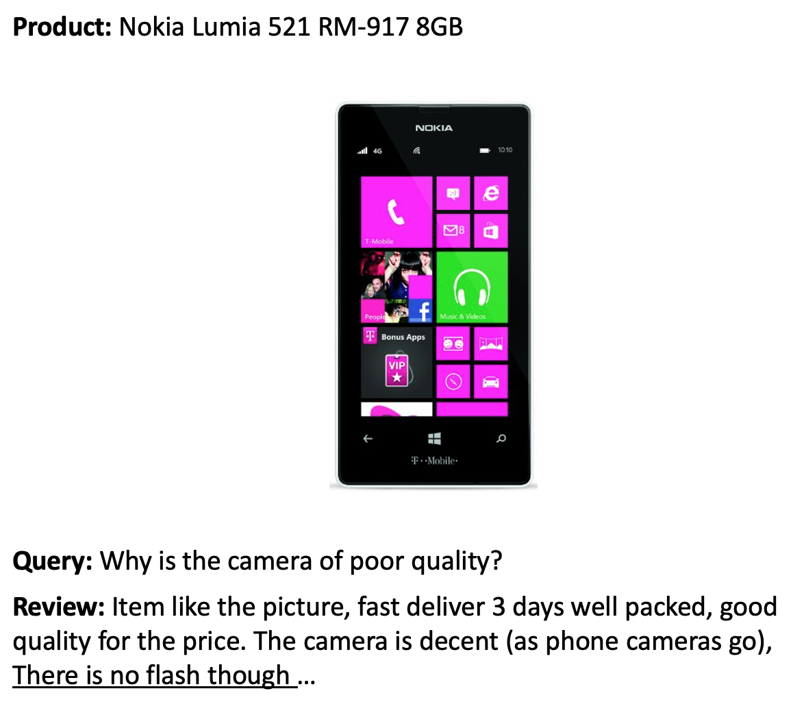
Figure 2-2. A question about a product and the corresponding review. The answer span is underlined.
The interesting aspect of this dataset is that most of the questions and answers are subjective, that is, they depend on the personal experience of the users. The example in Figure 2-2 shows why this feature is potentially more difficult than finding answers to factual questions like “What is the currency of the United Kingdom?”. First, the query is about “poor quality”, which is subjective and depends on the user’s definition of quality. Second, important parts of the query do not appear in the review at all, which means it cannot be answered with shortcuts like keyword-search or paraphrasing the input question. These features make SubjQA a realistic dataset to benchmark our review-based QA models on, since user-generated content like that shown in Figure 2-2 resembles what we might encounter in the wild.
Note
QA systems are usually categorized by the domain of data that they have access to when responding to a query. Closed-domain QA deals with questions about a narrow topic (e.g. a single product category), while open-domain deals with questions about almost anything (e.g. Amazon’s whole product catalogue). In general, closed-domain QA involves searching through fewer documents than the open-domain case.
For our use case, we’ll focus on building a QA system for the Electronics domain, so to get started let’s download the dataset from the Hugging Face Hub:
fromdatasetsimportload_datasetsubjqa=load_dataset("subjqa","electronics")
Next, let’s convert the dataset to the pandas format so
that we can explore it a bit more easily:
importpandasaspdsubjqa.set_format("pandas")# Flatten the nested dataset columns for easy accessdfs={split:ds[:]forsplit,dsinsubjqa.flatten().items()}forsplit,dfindfs.items():(f"Number of questions in {split}: {df['id'].nunique()}")
Number of questions in train: 1295
Number of questions in test: 358
Number of questions in validation: 255
Notice that the dataset is relatively small, with only 1,908 examples in total. This simulates a real-world scenario, since getting domain experts to label extractive QA datasets is labor-intensive and expensive. For example, the CUAD dataset for extractive QA on legal contracts is estimated to have a value of $2 million to account for the legal expertise and training of the annotators!
There are quite a few columns in the SubjQA dataset, but the most interesting ones for building our QA system are shown in Table 2-1.
| Column Name | Description |
|---|---|
title |
The Amazon Standard Identification Number (ASIN) associated with each product |
question |
The question |
answers.answer_text |
The span of text in the review labeled by the annotator |
answers.answer_start |
The start character index of the answer span |
context |
The customer review |
Let’s focus on these columns and take a look at a few of the
training examples by using the DataFrame.sample function to select a
random sample:
qa_cols=["title","question","answers.text","answers.answer_start","context"]sample_df=dfs["train"][qa_cols].sample(2,random_state=7)display_df(sample_df,index=False)
| title | question | answers.text | answers.answer_start | context |
|---|---|---|---|---|
| B005DKZTMG | Does the keyboard lightweight? | [this keyboard is compact] | [215] | I really like this keyboard. I give it 4 stars because it doesn’t have a CAPS LOCK key so I never know if my caps are on. But for the price, it really suffices as a wireless keyboard. I have very large hands and this keyboard is compact, but I have no complaints. |
| B00AAIPT76 | How is the battery? | [] | [] | I bought this after the first spare gopro battery I bought wouldn’t hold a charge. I have very realistic expectations of this sort of product, I am skeptical of amazing stories of charge time and battery life but I do expect the batteries to hold a charge for a couple of weeks at least and for the charger to work like a charger. In this I was not disappointed. I am a river rafter and found that the gopro burns through power in a hurry so this purchase solved that issue. the batteries held a charge, on shorter trips the extra two batteries were enough and on longer trips I could use my friends JOOS Orange to recharge them.I just bought a newtrent xtreme powerpak and expect to be able to charge these with that so I will not run out of power again. |
From these examples we can make a few observations. First, the questions
are not grammatically correct, which is quite common in the FAQ sections
of e-commerce websites. Second, an empty answers.text entry denotes
questions whose answer cannot be found in the review. Finally, we can
use the start index and length of the answer span to slice out the span
of text in the review that corresponds to the answer:
start_idx=sample_df["answers.answer_start"].iloc[0][0]end_idx=start_idx+len(sample_df["answers.text"].iloc[0][0])sample_df["context"].iloc[0][start_idx:end_idx]
'this keyboard is compact'
Next, let’s get a feel for what types of questions are in the training set by counting the questions that begin with a few common starting words:
counts={}question_types=["What","How","Is","Does","Do","Was","Where","Why"]forqinquestion_types:counts[q]=dfs["train"]["question"].str.startswith(q).value_counts()[True]pd.Series(counts).sort_values().plot.barh();
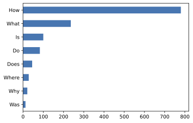
We can see that questions beginning with “How”, “What”, and “Is” are the most common ones, so let’s have a look at some examples:
forquestion_typein["How","What","Is"]:forquestionin(dfs["train"].query(f"question.str.startswith('{question_type}')").sample(n=3,random_state=42)['question']):(question)()
How is the camera?
How do you like the control?
How fast is the charger?

What is direction?
What is the quality of the construction of the bag?
What is your impression of the product?

Is this how zoom works?
Is sound clear?
Is it a wireless keyboard?
To round out our exploratory analysis, let’s visualize the distribution of reviews associated with each product in the training set:
fig,ax=plt.subplots()(dfs["train"].groupby("title")["review_id"].nunique().hist(bins=50,alpha=0.5,grid=False,ax=ax))plt.xlabel("Number of reviews per product")plt.ylabel("Count");

Here we see that most products have one review, while one has over fifty. In practice, our labeled dataset would be a subset of a much larger, unlabeled corpus, so this distribution presumably reflects the limitations of the annotation procedure. Now that we’ve explored our dataset a bit, let’s dive into understanding how transformers can extract answers from text.
Extracting Answers from Text
The first thing we’ll need for our QA system is to find a way to identify potential answers as a span of text in a customer review. For example, if a we have a question like “Is it waterproof?” and the review passage is “This watch is waterproof at 30m depth”, then the model should output “waterproof at 30m”. To do this we’ll need to understand how to:
-
Frame the supervised learning problem.
-
Tokenize and encode text for QA tasks.
-
Deal with long passages that exceed a model’s maximum context size.
Let’s start by taking a look at how to frame the problem.
Span Classification
The most common way to extract answers from text is by framing the problem as a span classification task, where the start and end tokens of an answer span act as the labels that a model needs to predict. This process is illustrated in Figure 2-3.
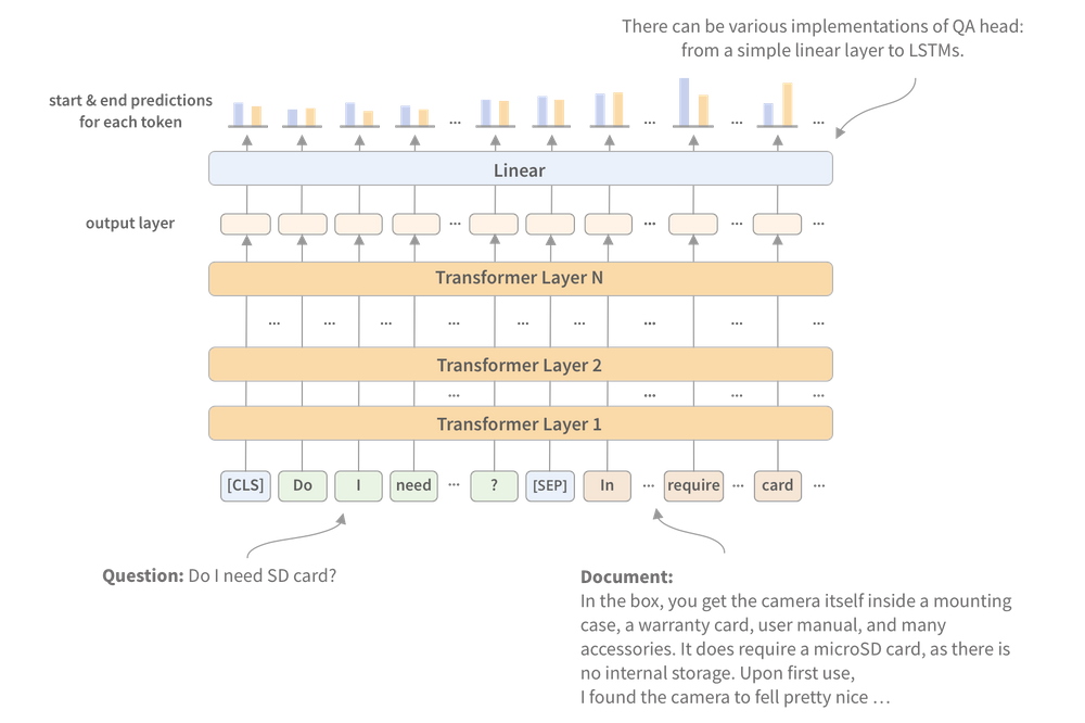
Figure 2-3. The span classification head for QA tasks.
Since our training set is relatively small with only 1,295 examples, a good strategy is to start with a language model that has already been fine-tuned on a large-scale QA dataset like the Stanford Question Answering Dataset (SQuAD).4 In general, these models have strong reading comprehension capabilities and serve as a good baseline upon which to build a more accurate system. You can find a list of extractive QA models by navigating to the Hugging Face Hub and searching for “squad” under the Models tab.
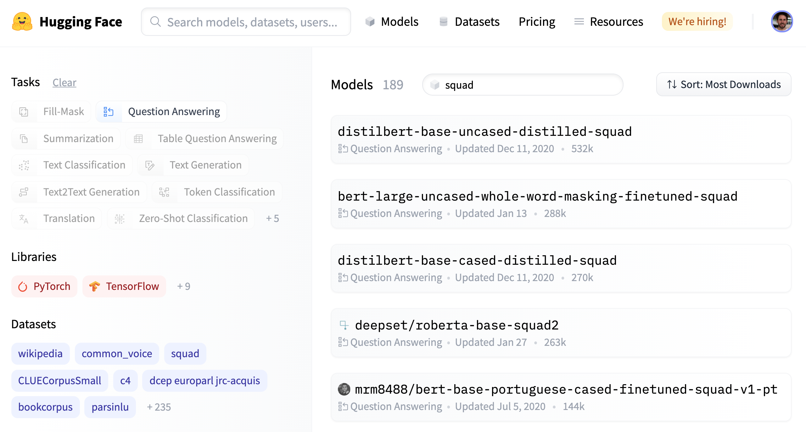
Figure 2-4. A selection of extractive QA models on the Hugging Face Hub.
As shown in Figure 2-4, there are more than 180 QA models to choose from, so which one should we pick? Although the answer depends on various factors like whether your corpus is mono- or multilingual, and the constraints of running the model in a production environment, Table 2-2 collects a few models that provide a good foundation to build on.
| Transformer | Description | Number of Parameters | F1 Score on SQuAD 2.0 |
|---|---|---|---|
MiniLM |
A distilled version of BERT-base that preserves 99% of the performance while being twice as fast |
66M |
79.5 |
RoBERTa-base |
RoBERTa models have better performance than their BERT counterparts and can be fine-tuned on most QA datasets using a single GPU |
125M |
83.0 |
ALBERT-XXL |
State-of-the-art performance on SQuAD 2.0, but computationally intensive and difficult to deploy |
235M |
88.1 |
XLM-RoBERTa-large |
Multilingual model for 100 languages with strong zero-shot performance |
570M |
83.8 |
Tokenizing Text for QA
For the purposes of this chapter, we’ll use a fine-tuned MiniLM model5 since it is fast to train and will allow us to quickly iterate on the techniques that we’ll be exploring. As usual, the first thing we need is a tokenizer to encode our texts so let’s load the model checkpoint from the Hugging Face Hub as follows:
fromtransformersimportAutoTokenizermodel_ckpt="deepset/minilm-uncased-squad2"tokenizer=AutoTokenizer.from_pretrained(model_ckpt)
To see the model in action, let’s first try to extract an answer from a short passage of text. In extractive QA tasks, the inputs are provided as (question, context) tuples, so we pass them both to the tokenizer as follows:
question="How much music can this hold?"context="""An MP3 is about 1 MB/minute, so about 6000 hours depending onfile size."""inputs=tokenizer(question,context,return_tensors="pt")
Here we’ve returned torch.Tensor objects since
we’ll need them to run the forward pass through the model.
If we view the tokenized inputs as a table:
| input_ids | 101 | 2129 | 2172 | 2189 | 2064 | 2023 | ... | 5834 | 2006 | 5371 | 2946 | 1012 | 102 |
|---|---|---|---|---|---|---|---|---|---|---|---|---|---|
| token_type_ids | 0 | 0 | 0 | 0 | 0 | 0 | ... | 1 | 1 | 1 | 1 | 1 | 1 |
| attention_mask | 1 | 1 | 1 | 1 | 1 | 1 | ... | 1 | 1 | 1 | 1 | 1 | 1 |
we can also see the familiar input_ids and attention_mask tensors,
while the token_type_ids tensor indicates which part of the inputs
corresponds to the question and context (a 0 indicates a question token,
a 1 indicates a context token).6 To
understand how the tokenizer formats the inputs for QA tasks,
let’s decode the input_ids tensor:
tokenizer.decode(inputs["input_ids"][0])
'[CLS] how much music can this hold? [SEP] an mp3 is about 1 mb / minute, so
 > about 6000 hours depending on file size. [SEP]'
We see that for each QA example, the inputs take the format:
[CLS] question tokens [SEP] context tokens [SEP]
where the location of the first [SEP] token is determined by the
token_type_ids. Now that our text is tokenized, we just need to
instantiate the model with a QA head and run the inputs through the
forward pass:
fromtransformersimportAutoModelForQuestionAnsweringmodel=AutoModelForQuestionAnswering.from_pretrained(model_ckpt)outputs=model(**inputs)
As illustrated in Figure 2-3, the QA head corresponds to a linear layer that takes the hidden-states from the encoder7 and computes the logits for the start and end spans. To convert the outputs into an answer span, we first need to get the logits for the start and end tokens:
start_scores=outputs.start_logitsend_scores=outputs.end_logits
As illustrated in Figure 2-5, each input token is given a score by the model, with larger, positive scores corresponding to more likely candidates for the start and end tokens. In this example we can see that the model assigns the highest start token scores to the numbers “1” and “6000” which makes sense since our question is asking about a quantity. Similarly, we see that the highest scored end tokens are “minute” and “hours”.

Figure 2-5. Predicted logits for the start and end tokens. The token with the highest score is colored in orange.
To get the final answer, we can compute the argmax over the start and end token scores and then slice the span from the inputs. The following code does these steps and decodes the result so we can print the resulting text:
importtorchstart_idx=torch.argmax(start_scores)end_idx=torch.argmax(end_scores)+1answer_span=inputs["input_ids"][0][start_idx:end_idx]answer=tokenizer.decode(answer_span)(f"Question: {question}")(f"Answer: {answer}")
Question: How much music can this hold?
Answer: 6000 hours
Great, it worked! In Transformers, all of these pre-processing and
post-processing steps are conveniently wrapped in a dedicated
QuestionAnsweringPipeline. We can instantiate the pipeline by passing
our tokenizer and fine-tuned model as follows:
fromtransformersimportQuestionAnsweringPipelinepipe=QuestionAnsweringPipeline(model=model,tokenizer=tokenizer)pipe(question=question,context=context,topk=3)
[{'score': 0.26516082882881165,
  'start': 38,
  'end': 48,
  'answer': '6000 hours'},
 {'score': 0.2208300083875656,
  'start': 16,
  'end': 48,
  'answer': '1 MB/minute, so about 6000 hours'},
 {'score': 0.10253595560789108,
  'start': 16,
  'end': 27,
  'answer': '1 MB/minute'}]
In addition to the answer, the pipeline also returns the
model’s probability estimate (obtained by taking a softmax
over the logits), which is handy when we want to compare multiple
answers within a single context. We’ve also shown that the
model can predict multiple answers by specifying the topk parameter.
Sometimes, it is possible to have questions for which no answer is
possible, like the empty answers.answer_start examples in SubjQA. In
these cases, the model will assign a high start and end score to the
[CLS] token and the pipeline maps this output to an empty string:
pipe(question="Why is there no data?",context=context,handle_impossible_answer=True)
{'score': 0.9068416357040405, 'start': 0, 'end': 0, 'answer': ''}
Note
In our simple example, we obtained the start and end indices by taking the argmax of the corresponding logits. However, this heuristic can produce out-of-scope answers (e.g. it can select tokens that belong to the question instead of the context), so in practice the pipeline computes the best combination of start and end indices subject to various constraints such as being in-scope, the start indices have to precede end indices and so on.
Dealing With Long Passages
One subtlety faced by reading comprehension models is that the context often contains more tokens than the maximum sequence length of the model, which is usually a few hundred tokens at most. As illustrated in Figure 2-6, a decent portion of the SubjQA training set contains question-context pairs that won’t fit within the model’s context.

Figure 2-6. Distribution of tokens for each question-context pair in the SubjQA training set.
For other tasks like text classification, we simply truncated long texts
under the assumption that enough information was contained in the
embedding of the [CLS] token to generate accurate predictions. For QA
however, this strategy is problematic because the answer to a question
could lie near the end of the context and would be removed by
truncation. As illustrated in Figure 2-7, the standard
way to deal with this is to apply a sliding window across the inputs,
where each window contains a passage of tokens that fit in the
model’s context.

Figure 2-7. How the sliding window creates multiple question-context pairs for long documents.
In Transformers, the sliding window is enabled by setting
return_overflowing_tokens=True in the tokenizer, with the size of the
sliding window controlled by the max_seq_length argument and the size
of the stride controlled by doc_stride. Let’s grab the
first example from our training set and define a small window to
illustrate how this works:
example=dfs["train"].iloc[0][["question","context"]]tokenized_example=tokenizer(example["question"],example["context"],return_overflowing_tokens=True,max_length=100,stride=25)
In this case we now get a list of input_ids, one for each window.
Let’s check the number of tokens we have in each window:
foridx,windowinenumerate(tokenized_example["input_ids"]):(f"Window #{idx} has {len(window)} tokens")
Window #0 has 100 tokens
Window #1 has 88 tokens
Finally we can see where two windows overlap by decoding the inputs:
forwindowintokenized_example["input_ids"]:(tokenizer.decode(window),"")
[CLS] how is the bass? [SEP] i have had koss headphones in the past, pro 4aa and
 > qz - 99. the koss portapro is portable and has great bass response. the work
 > great with my android phone and can be " rolled up " to be carried in my
 > motorcycle jacket or computer bag without getting crunched. they are very
 > light and don't feel heavy or bear down on your ears even after listening to
 > music with them on all day. the sound is [SEP]

[CLS] how is the bass? [SEP] and don't feel heavy or bear down on your ears even
 > after listening to music with them on all day. the sound is night and day
 > better than any ear - bud could be and are almost as good as the pro 4aa.
 > they are " open air " headphones so you cannot match the bass to the sealed
 > types, but it comes close. for $ 32, you cannot go wrong. [SEP]
Now that we have some intuition about how QA models can extract answers from text, let’s look at the other components we need to build an end-to-end QA pipeline.
Using Haystack to Build a QA Pipeline
In our simple answer extraction example, we provided both the question and the context to the model. However, in reality our system’s users will only provide a question about a product, so we need some way of selecting relevant passages from among all the reviews in our corpus. One way to do this would be to concantenate all the reviews of a given product together and feed them to the model as a single, long context. Although simple, the drawback of this approach is that the context can become extremely long and thereby introduce an unacceptable latency for our users’ queries. For example, let’s suppose that on average, each product has 30 reviews and each review takes 100 milliseconds to process. If we need to process all the reviews to get an answer, this would give an average latency of three seconds per user query - much too long for e-commerce websites!
To handle this, modern QA systems are typically based on the Retriever-Reader architecture, which has two main components:
- Retriever
-
Responsible for retrieving relevant documents for a given query. Retrievers are usually categorized as sparse or dense. Sparse Retrievers use sparse vector representations of the documents to measure which terms match with a query. Dense Retrievers use encoders like transformers or LSTMs to encode a query and document in two respective vectors of identical length. The relevance of a query and a document is then determined by computing an inner product of the vectors.
- Reader
-
Responsible for extracting an answer from the documents provided by the Retriever. The Reader is usually a reading comprehension model, although we’ll see at the end of the chapter examples of models that can generate free-form answers.
As illustrated in Figure 2-9, there can also be other components that apply post-processing to the documents fetched by the Retriever or to the answers extracted by the Reader. For example, the retrieved documents may need re-ranking to eliminate noisy or irrelevant ones that can confuse the Reader. Similarly, post-processing of the Reader’s answers is often needed when the correct answer comes from various passages in a long document.
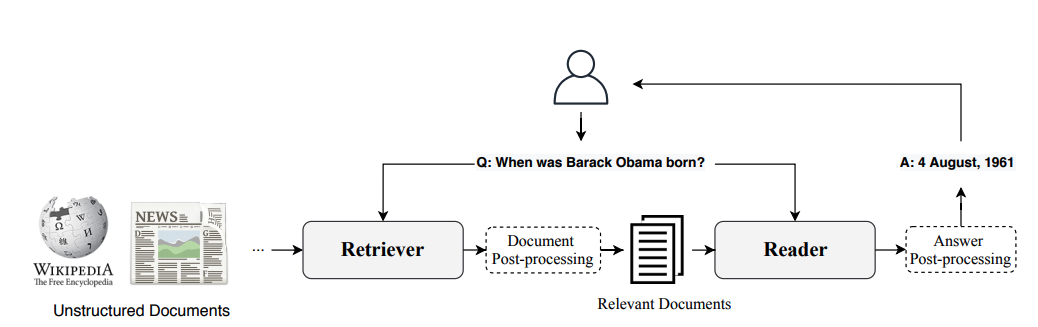
Figure 2-9. The Retriever-Reader architecture for modern QA systems.
To build our QA system, we’ll use the
Haystack library which is developed by
deepset, a German company focused on NLP. The
advantage of using Haystack is that it’s based on the
Retriever-Reader architecture, abstracts much of the complexity involved
in building these systems, and integrates tightly with Transformers. You
can install Haystack with the following pip command:
pipinstallfarm-haystack
In addition to the Retriever and Reader, there are two more components involved when building a QA pipeline with Haystack:
- Document store
-
A document-oriented database that stores documents and metadata which are provided to the Retriever at query time.
- Pipeline
-
Combines all the components of a QA system to enable custom query flows, merging documents from multiple Retrievers, and more.
In this section we’ll look at how we can use these components to quickly build a prototype QA pipeline, and later examine how we can improve its performance.
Initializing a Document Store
In Haystack, there are various document stores to choose from and each one can be paired with a dedicated set of Retrievers. This is illustrated in Table 2-3, where the compatibility of sparse (TF-IDF, BM25) and dense (Embedding, DPR) Retrievers is shown for each of the available document stores.
| In Memory | Elasticsearch | FAISS | Milvus | |
|---|---|---|---|---|
TF-IDF |
Yes |
Yes |
No |
No |
BM25 |
No |
Yes |
No |
No |
Embedding |
Yes |
Yes |
Yes |
Yes |
DPR |
Yes |
Yes |
Yes |
Yes |
Since we’ll be exploring both sparse and dense retrievers in
this chapter, we’ll use the ElasticsearchDocumentStore
which is compatible with both retriever types. Elasticsearch is a search
engine that is capable of handling a diverse range of data, including
textual, numerical, geospatial, structured, and unstructured. Its
ability to store huge volumes of data and quickly filter it with
full-text search features makes it especially well suited for developing
QA systems. It also has the advantage of being the industry standard for
infrastructure analytics, so there’s a good chance your
company already has a cluster that you can work with.
To initialize the document store, we first need to download and install
Elasticsearch. By following Elasticsearch’s
guide,
let’s grab the latest release for Linux10 with
wget and unpack it with the tar shell command:
url="""https://artifacts.elastic.co/downloads/elasticsearch/elasticsearch-7.9.2-linux-x86_64.tar.gz"""!wget-nc-q{url}!tar-xzfelasticsearch-7.9.2-linux-x86_64.tar.gz
Next we need to start the Elasticsearch server. Since we’re
running all the code in this book within Jupyter notebooks,
we’ll need to use Python’s subprocess.Popen
module to spawn a new process. While we’re at it,
let’s also run the subprocess in the background using the
chown shell command:
importosfromsubprocessimportPopen,PIPE,STDOUT# Run Elasticsearch as a background process!chown-Rdaemon:daemonelasticsearch-7.9.2es_server=Popen(args=['elasticsearch-7.9.2/bin/elasticsearch'],stdout=PIPE,stderr=STDOUT,preexec_fn=lambda:os.setuid(1))# Wait until Elasticsearch has started!sleep30
In the Popen module, the args specify the program we wish to
execute, while stdout=PIPE creates a new pipe for the standard output,
and stderr=STDOUT collects the errors in the same pipe. The
preexec_fn argument specifies the ID of the subprocess we wish to use.
By default, Elasticsearch runs locally on port 9200, so we can test the
connection by sending a HTTP request to localhost:
!curl-XGET"localhost:9200/?pretty"
{
  "name" : "n1hikaoslz",
  "cluster_name" : "elasticsearch",
  "cluster_uuid" : "2QZjiLIMSJKiGFLyatR_NQ",
  "version" : {
    "number" : "7.9.2",
    "build_flavor" : "default",
    "build_type" : "tar",
    "build_hash" : "d34da0ea4a966c4e49417f2da2f244e3e97b4e6e",
    "build_date" : "2020-09-23T00:45:33.626720Z",
    "build_snapshot" : false,
    "lucene_version" : "8.6.2",
    "minimum_wire_compatibility_version" : "6.8.0",
    "minimum_index_compatibility_version" : "6.0.0-beta1"
  },
  "tagline" : "You Know, for Search"
}
Now that our Elasticsearch server is up and running, the next thing to do is instantiate the document store:
fromhaystack.document_store.elasticsearchimportElasticsearchDocumentStore# Return the document embedding for later use with dense Retrieverdocument_store=ElasticsearchDocumentStore(return_embedding=True)
05/11/2021 17:06:50 - INFO - faiss.loader -   Loading faiss with AVX2 support.
05/11/2021 17:06:50 - INFO - faiss.loader -   Loading faiss.
By default, ElasticsearchDocumentStore creates two indices on
Elasticsearch: one called document for (you guessed it) storing
documents, and another called label for storing the annotated answer
spans. For now, we’ll just populate the document index
with the SubjQA reviews, and Haystack’s document stores
expect a list of dictionaries with text and meta keys as follows:
{
    "text": "<the-context>",
    "meta": {
        "field_01": "<additional-metadata>",
        "field_02": "<additional-metadata>",
        ...
    }
}
The fields in meta can be used for applying filters during retrieval,
so for our purposes we’ll include the item_id and
q_review_id columns of SubjQA so we can filter by product and question
ID, along with the corresponding training split. We can then loop
through the examples in each DataFrame and add them to the index with
the write_documents function as follows:
forsplit,dfindfs.items():# Exclude duplicate reviewsdocs=[{"text":row["context"],"meta":{"item_id":row["title"],"qid":row["id"],"split":split}}for_,rowindf.drop_duplicates(subset="context").iterrows()]document_store.write_documents(docs,index="document")(f"Loaded {document_store.get_document_count()} documents")
Loaded 1875 documents
Great, we’ve loaded all our reviews into an index! To search the index we’ll need a Retriever, so let’s look at how we can intialize one for Elasticsearch.
Initializing a Retriever
The Elasticsearch document store can be paired with any of the Haystack retrievers, so let’s start by using a sparse retriever based on BM25 (short for “Best Match 25”). BM25 is an improved version of the classic TF-IDF metric and represents the question and context as sparse vectors that can be searched efficiently on Elasticsearch. The BM25 score measures how much matched text is about a search query and improves on TF-IDF by saturating TF values quickly and normalizing the document length so that short documents are favoured over long ones.11
In Haystack, the BM25 Retriever is included in ElasticsearchRetriever,
so let’s initialize this class by specifying the document
store we wish to search over:
fromhaystack.retriever.sparseimportElasticsearchRetrieveres_retriever=ElasticsearchRetriever(document_store=document_store)
Next, let’s look at a simple query for a single electronics
product in the training set. For review-based QA systems like ours,
it’s important to restrict the queries to a single item
because otherwise the Retriever would source reviews about products that
are not related to a user’s query. For example, asking “Is
the camera quality any good?” without a product filter could return
reviews about phones, when the user might be asking about a specific
laptop camera instead. By themselves, the ASIN values in our dataset are
a bit cryptic, but we can decipher them with online tools like
amazon ASIN or by simply appending the value
of item_id to the www.amazon.com/dp/ URL. The item ID below
corresponds to one of Amazon’s Fire tablets, so
let’s use the Retriever’s retrieve function to
ask if it’s any good for reading with:
item_id="B0074BW614"query="Is it good for reading?"retrieved_docs=es_retriever.retrieve(query=query,top_k=3,filters={"item_id":[item_id],"split":["train"]})
Here we’ve specified how many documents to return with the
top_k argument and applied a filter on both the item_id and split
keys that were included in the meta field of our documents. Each
element of retrieved_docs is a Haystack Document object that is used
to represent documents and includes the Retriever’s query
score along with other metadata. Let’s have a look at one of
the retrieved documents:
retrieved_docs[0]
{'text': 'This is a gift to myself.  I have been a kindle user for 4 years and
 > this is my third one.  I never thought I would want a fire for I mainly use
 > it for book reading.  I decided to try the fire for when I travel I take my
 > laptop, my phone and my iPod classic.  I love my iPod but watching movies on
 > the plane with it can be challenging because it is so small. Laptops battery
 > life is not as good as the Kindle.  So the Fire combines for me what I needed
 > all three to do. So far so good.', 'id':
 > '4d209402-0f0e-4c90-a5ff-99dc15aabba1', 'score': 6.243799, 'probability':
 > 0.6857824513476455, 'question': None, 'meta': {'item_id': 'B0074BW614',
 > 'qid': '868e311275e26dbafe5af70774a300f3', 'split': 'train'}, 'embedding':
 > None}
In addition to the document’s text, we can see the score
that Elasticsearch computed for its relevance to the query (larger
scores imply a better match). Under the hood, Elasticsearch relies on
Lucene for indexing and search, so by
default it uses Lucene’s practical scoring function. You
can find the nitty gritty details behind the scoring function in the
Elasticsearch
documentation, but in brief terms the scoring function first filters
the candidate documents by applying a boolean test (does the document
match the query?), and then applies a similarity metric
that’s based on representing both the document and query as
vectors.
Now that we have a way to retrieve relevant documents, the next thing we need is a way to extract answers from them. This is where the Reader comes in, so let’s take a look at how we can load our MiniLM model in Haystack.
Initializing a Reader
In Haystack, there are two types of Readers one can use to extract answers from a given context:
FARMReader-
Based on deepset’s FARM framework for fine-tuning and deploying transformers. Compatible with models trained using Transformers and can load models directly from the Hugging Face Hub.
TransformersReader-
Based on the
QuestionAnsweringPipelinefrom Transformers. Suitable for running inference only.
Although both Readers handle a model’s weights in the same way, there are some differences in the way the predictions are converted to produce answers:
-
In Transformers, the
QuestionAnsweringPipelinenormalizes the start and end logits with a softmax in each passage. This means that it is only meaningful to compare answer scores between answers extracted from the same passage, where the probabilities sum to one. For example, an answer score of 0.9 from one passage is not necessarily better than a score of 0.8 in another. In FARM, the logits are not normalized, so inter-passage answers can be compared more easily. -
The
TransformersReadersometimes predicts the same answer twice, but with different scores. This can happen in long contexts if the answer lies across two overlapping windows. In FARM, these duplicates are removed.
Since we will be fine-tuning the Reader later in the chapter,
we’ll use the FARMReader. Similar to Transformers, to load
the model we just need to specify the MiniLM checkpoint on the Hugging
Face Hub along with some QA-specific arguments:
fromhaystack.reader.farmimportFARMReadermodel_ckpt="deepset/minilm-uncased-squad2"max_seq_length,doc_stride=384,128reader=FARMReader(model_name_or_path=model_ckpt,progress_bar=False,max_seq_len=max_seq_length,doc_stride=doc_stride,return_no_answer=True)
Note
It is also possible to fine-tune a reading comprehension model directly in Transformers and then load it in TransformersReader to run inference. For details on how to do the fine-tuning step, see the question-answering tutorial in the Transformers’ Big Table of Tasks.
In FARMReader, the behavior of the sliding window is controlled by the
same max_seq_length and doc_stride arguments that we saw for the
tokenizer, and we’ve used the values from the MiniLM paper.
As a sanity check, let’s now test the Reader on our simple
example from earlier:
reader.predict_on_texts(question=question,texts=[context],top_k=1)
{'query': 'How much music can this hold?',
 'no_ans_gap': 12.648080229759216,
 'answers': [{'answer': '6000 hours',
   'score': 10.699615478515625,
   'probability': 0.3988127112388611,
   'context': 'An MP3 is about 1 MB/minute, so about 6000 hours depending on
 > file size.',
   'offset_start': 38,
   'offset_end': 48,
   'offset_start_in_doc': 38,
   'offset_end_in_doc': 48,
   'document_id': 'e17cdee5-fe11-4d25-97d4-72aefa0e2101'}]}
Great, the Reader appears to be working as expected, so next let’s tie together all our components using one of Haystack’s pipelines.
Putting It All Together
Haystack provides a Pipeline abstraction that allows us to combine
Retrievers, Readers, and other components together as a graph that can
be easily customized for each use case. There are also predefined
pipelines analogous to those in Transformers, but specialized for QA
systems. In our case, we’re interested in extracting answers
so we’ll use the ExtractiveQAPipeline which takes a single
Retriever-Reader pair as its arguments:
fromhaystack.pipelineimportExtractiveQAPipelinepipe=ExtractiveQAPipeline(reader,es_retriever)
Each Pipeline has a run function that specifies how the query flow
should be executed. For ExtractiveQAPipeline we just need to pass the
query, the number of documents to retrieve with top_k_retriever, and
number of answers to extract from these documents with top_k_reader.
In our case, we also need to specify a filter over the item ID which can
be done using the filters argument as we did with the Retriever
earlier. Let’s run a simple example using our question about
the Amazon Fire tablet again, but this time returning the extracted
answers:
n_answers=3preds=pipe.run(query=query,top_k_retriever=3,top_k_reader=n_answers,filters={"item_id":[item_id],"split":["train"]})(f"Question: {preds['query']}","")foridxinrange(n_answers):(f"Answer {idx+1}: {preds['answers'][idx]['answer']}")(f"Review snippet: ...{preds['answers'][idx]['context']}...")("")
Question: Is it good for reading?

Answer 1: I mainly use it for book reading
Review snippet: ... is my third one.  I never thought I would want a fire for I
 > mainly use it for book reading.  I decided to try the fire for when I travel
 > I take my la...


Answer 2: the larger screen compared to the Kindle makes for easier reading
Review snippet: ...ght enough that I can hold it to read, but the larger screen
 > compared to the Kindle makes for easier reading. I love the color, something
 > I never thou...


Answer 3: it is great for reading books when no light is available
Review snippet: ...ecoming addicted to hers! Our son LOVES it and it is great
 > for reading books when no light is available. Amazing sound but I suggest
 > good headphones t...
Great, we now have an end-to-end QA system for Amazon product reviews! This is a good start, but notice that the second and third answer are closer to what the question is actually asking. To do better, we’ll first need some metrics to quantify the performance of the Retriever and Reader. Let’s take a look.
Improving Our QA Pipeline
Although much of the recent research on QA has focused on improving reading comprehension models, in practice it doesn’t matter how good your Reader is if the Retriever can’t find the relevant documents in the first place! In particular, the Retriever sets an upper bound on the performance of the whole QA system, so it’s important to make sure it’s doing a good job. With this in mind, let’s start by introducing metrics to evaluate the Retriever and comparing the performance of sparse and dense representations.
Evaluating the Retriever
A common metric for evaluating Retrievers is recall, which measures
the fraction of all relevant documents that are retrieved. In this
context, relevant simply means whether the answer is present in a
passage of text or not, so given a set of questions, we can compute
recall by counting the number of times an answer appears in the
top-
Note
A complementary metric to recall is mean average precision (mAP), which rewards Retrievers that can place the correct answers higher up in the document ranking.
In Haystack there are two ways to evaluate Retrievers:
-
Use the Retriever’s in-built
evalfunction. This can be used for both open- and closed-domain QA, but not for datasets like SubjQA where each document is paired with a single product and we need to filter by product ID for every query. -
Build a custom
Pipelinethat combines a Retriever with theEvalRetrieverclass. This enables the possibility to implement custom metrics and query flows.
Since we need to evaluate the recall per product and then aggregate
across all products, we’ll opt for the second approach. Each
node in the Pipeline graph represents a class that takes some inputs
and produces some ouputs via a run function:
classPipelineNode:def__init__(self):self.outgoing_edges=1defrun(self,**kwargs):...return(outputs,"outgoing_edge_name")
Here kwargs corresponds to the outputs from the previous node in the
graph, which is manipulated within run to return a tuple of the
outputs for the next node, along with a name for the outgoing edge. The
only other requirement is to include an outgoing_edge attribute that
indicates the number of outputs from the node (in most cases
outgoing_edge=1 unless you have branches in the pipeline that route
the inputs according to some criterion).
In our case, we need a node to evaluate the Retriever, so
we’ll use the EvalRetriever class whose run function
keeps track of which documents have answers that match the ground truth.
With this class we can then build up a Pipeline graph by adding the
evaluation node after a node that represents the Retriever itself:
fromhaystack.pipelineimportPipelinefromhaystack.evalimportEvalRetrieverclassEvalRetrieverPipeline:def__init__(self,retriever):self.retriever=retrieverself.eval_retriever=EvalRetriever()pipe=Pipeline(pipeline_type="Query")pipe.add_node(component=self.retriever,name="ESRetriever",inputs=["Query"])pipe.add_node(component=self.eval_retriever,name="EvalRetriever",inputs=["ESRetriever"])self.pipeline=pipepipe=EvalRetrieverPipeline(es_retriever)
Notice that each node is given a name and a list of inputs. In most
cases, each node has a single outgoing edge, so we just need to include
the name of the previous node in inputs.
Now that we have our evaluation pipeline, we need to pass some queries
and their corresponding answers. To do this, we’ll add the
answers to a dedicated label index on our document store. Haystack
provides a Label object that represents the answer spans and their
metadata in a standardized fashion. To populate the label index,
we’ll first create a list of Labels objects by looping
over each question in the test set and extracting the matching answers
and additional metadata:
fromhaystackimportLabellabels=[]for_,rowindfs["test"].iterrows():iflen(row["answers.text"]):foranswerinrow["answers.text"]:label=Label(question=row["question"],answer=answer,origin=row["id"],document_id=row["id"],model_id=row["title"],no_answer=False,is_correct_answer=True,is_correct_document=True)labels.append(label)else:label=Label(question=row["question"],answer="",origin=row["id"],document_id=row["id"],model_id=row["title"],is_correct_answer=True,is_correct_document=True,no_answer=False)labels.append(label)
If we peek at one of these labels
labels[0]
{'id': '00dccde9-76ef-4e46-a2be-dc2391f95363', 'created_at': None, 'updated_at':
 > None, 'question': 'What is the tonal balance of these headphones?', 'answer':
 > 'I have been a headphone fanatic for thirty years', 'is_correct_answer':
 > True, 'is_correct_document': True, 'origin':
 > 'd0781d13200014aa25860e44da9d5ea7', 'document_id':
 > 'd0781d13200014aa25860e44da9d5ea7', 'offset_start_in_doc': None, 'no_answer':
 > False, 'model_id': 'B00001WRSJ'}
we can see the question-answer pair along with an origin field that
contains the unique question ID so we can filter the document store per
question. We’ve also added the product ID to the model_id
field so we can filter the labels by product. Now that we have our
labels, we can write them to the label index on Elasticsearch as
follows:
document_store.write_labels(labels,index="label")(f"""Loaded {len(document_store.get_all_documents(index='label'))}question-answer pairs""")
Loaded 455 question-answer pairs
Next, we need to build up a mapping between our question IDs and
corresponding answers that we can pass to the pipeline. To get all the
labels, we can use the get_all_labels_aggregated function from the
document store that will aggregate all question-answer pairs associated
with a unique ID. This function returns a list of MultiLabel objects,
but in our case we only get one element since we’re
filtering by question ID, so we can build up a list of aggregated labels
as follows:
labels_agg=[]forqidindfs["test"]["id"].values:l=document_store.get_all_labels_aggregated(filters={"origin":[qid]})labels_agg.extend(l)
By peeking at one of these labels we can see that all the answer
associated with a given question are aggregated together in a
multiple_answers field:
labels_agg[14]
{'question': 'What is the cord like?', 'multiple_answers': ['the cord is either
 > too short and too long', 'cord is either too short and too long'],
 > 'is_correct_answer': True, 'is_correct_document': True, 'origin':
 > '47006bd3145448aabf92281eefdee61c', 'multiple_document_ids':
 > ['47006bd3145448aabf92281eefdee61c', '47006bd3145448aabf92281eefdee61c'],
 > 'multiple_offset_start_in_docs': [None, None], 'no_answer': False,
 > 'model_id': 'B000092YQW'}
Since we’ll soon evaluate both the Retriever and Reader in
the same run, we need to provide the gold labels for both components in
the Pipeline.run function. The simplest way to achieve this is by
creating a dictionary that maps the unique question ID with a dictionary
of labels, one for each component:
qid2label={l.origin:{"retriever":l,"reader":l}forlinlabels_agg}
We now have all the ingredients for evaluating the Retriever, so
let’s define a function that feeds each question-answers
pair associated with each product to the evaluation pipeline and tracks
the correct retrievals in our pipe object:
defrun_pipeline(pipeline,top_k_retriever=10,top_k_reader=4):forq,linqid2label.items():_=pipeline.pipeline.run(query=l["retriever"].question,top_k_retriever=top_k_retriever,top_k_reader=top_k_reader,labels=l,filters={"item_id":[l["retriever"].model_id],"split":["test"]})# Display Retriever metricsrun_pipeline(pipe,top_k_retriever=3)pipe.eval_retriever.()
Retriever
----------------
-
recall: 0.9525 (341 / 358)
Great, it works! Notice that we picked a specific value for
top_k_retriever to specify the number of documents to retrieve. In
general, increasing this parameter will improve the recall, but at the
expense of providing more documents to the Reader and slowing down the
end-to-end pipeline. To guide our decision on which value to pick,
we’ll create a function that loops over several
defevaluate_retriever(retriever,topk_values=[1,3,5,10,20]):topk_results={}fortopkintopk_values:# Create Pipelinep=EvalRetrieverPipeline(retriever)# Loop over each question-answers pair in test setrun_pipeline(p,top_k_retriever=topk)# Get metricstopk_results[topk]={"recall":p.eval_retriever.recall}returnpd.DataFrame.from_dict(topk_results,orient="index")es_topk_df=evaluate_retriever(es_retriever)
If we plot the results, we can see how the recall improves as we
increase
defplot_retriever_eval(dfs,retriever_names):fig,ax=plt.subplots()fordf,retriever_nameinzip(dfs,retriever_names):df.plot(y="recall",ax=ax,label=retriever_name)plt.xticks(df.index)plt.ylabel("Top-k Recall")plt.xlabel("k")plot_retriever_eval([es_topk_df],["BM25"])

From the plot we can see that there’s an inflection point
around
Dense Passage Retrieval
We’ve seen that we get almost perfect recall when our sparse
Retriever returns [CLS] token.
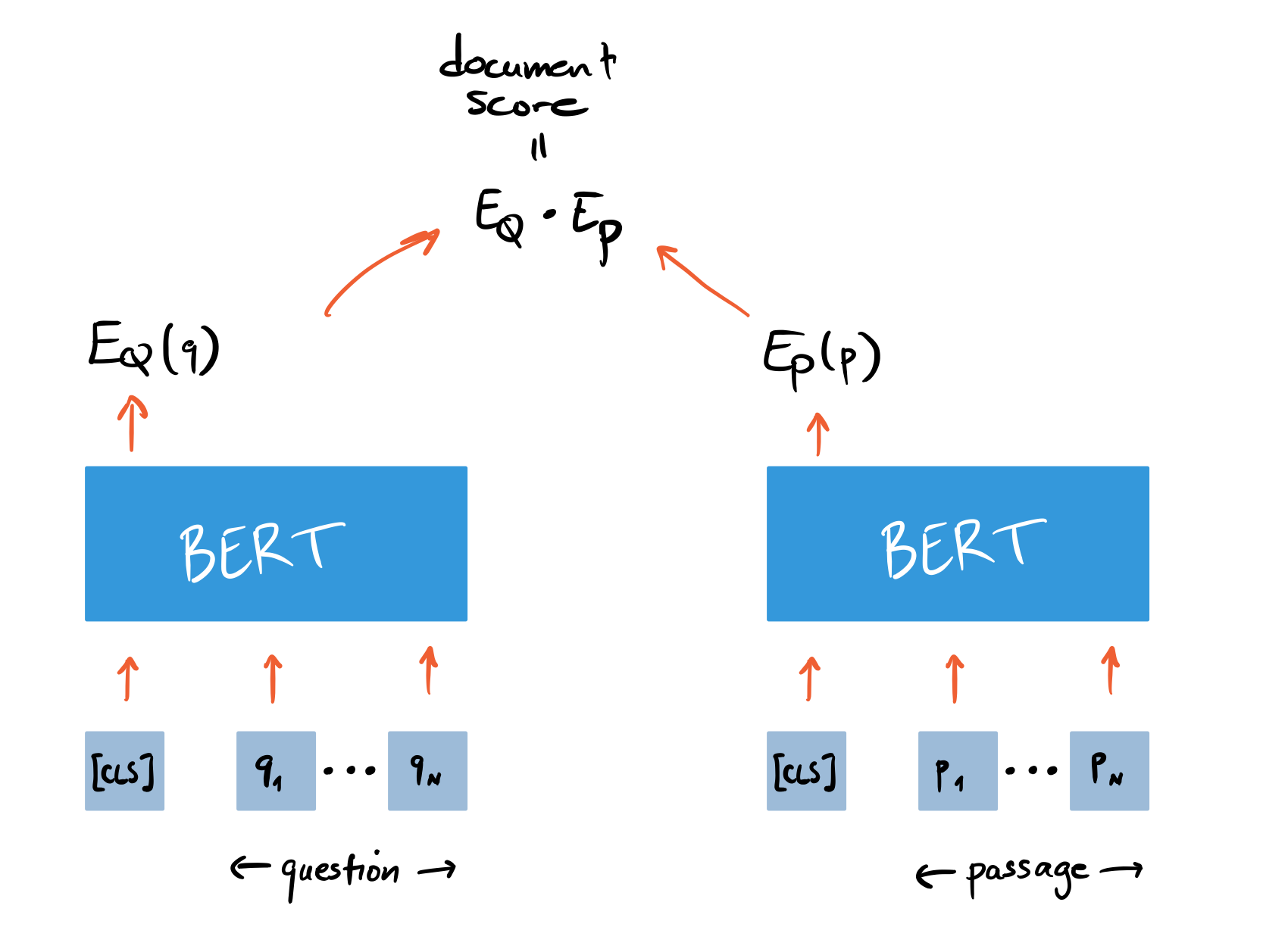
Figure 2-10. DPR’s bi-encoder architecture for computing the relevance of a document and query.
In Haystack, we can initialize a Retriever for DPR in a similar way we did for BM25. In addition to specifying the document store, we also need to pick the BERT encoders for the question and passage. These encoders are trained by giving them questions with relevant (positive) passages and irrelevant (negative) passages, where the goal is to learn that relevant question-passage pairs have a higher similarity. For our use case, we’ll use encoders that have been fine-tuned on the NQ corpus in this way:
fromhaystack.retriever.denseimportDensePassageRetrieverdpr_retriever=DensePassageRetriever(document_store=document_store,query_embedding_model="facebook/dpr-question_encoder-single-nq-base",passage_embedding_model="facebook/dpr-ctx_encoder-single-nq-base",embed_title=False)
Here we’ve also set embed_title=False since concatenating
the document’s title (i.e. item_id) doesn’t
provide any additional information because we filter per product. Once
we’ve initialized the dense Retriever, the next step is
iterate over all the indexed documents on our Elasticseach index and
apply the encoders to update the embedding representation. This can be
done as follows:
document_store.update_embeddings(retriever=dpr_retriever)
We’re now set to go! We can evaluate the dense Retriever in
the same way we did for BM25 and compare the top-
dpr_topk_df=evaluate_retriever(dpr_retriever)plot_retriever_eval([es_topk_df,dpr_topk_df],["BM25","DPR"])
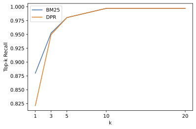
Here we can see that DPR does not provide a boost in recall over BM25
and saturates around
Tip
Performing similarity search of the embeddings can be sped up by using Facebook’s FAISS library as the document store. Similarly, the performance of the DPR Retriever can be improved by fine-tuning on the target domain.
Now that we’ve explored the evaluation of the Retriever, let’s turn to evaluating the Reader.
Evaluating the Reader
In extractive QA, there are two main metrics that are used for evaluating Readers:
- Exact Match (EM)
-
A binary metric that gives
-
We encountered this metric in Chapter 1 and it measures the harmonic mean of the precision and recall.
Let’s see how these metrics work by importing some helper functions from FARM and applying them to a simple example:
fromfarm.evaluation.squad_evaluationimportcompute_f1,compute_exactpred="about 6000 hours"label="6000 hours"(f"EM: {compute_exact(label, pred)}")(f"F1: {compute_f1(label, pred)}")
EM: 0
F1: 0.8
Under the hood, these functions first normalise the prediction and label by removing punctuation, fixing whitespace, and converting to lowercase. The normalized strings are then tokenized as a bag-of-words, before finally computing the metric at the token level. From this simple example we can see that EM is a much stricter metric than the F1 score: adding a single token to the prediction gives an EM of zero. On the other hand, the F1 score can fail to catch truly incorrect answers. For example, suppose our predicted answer span was “about 6000 dollars” then we get:
pred="about 6000 dollars"(f"EM: {compute_exact(label, pred)}")(f"F1: {compute_f1(label, pred)}")
EM: 0
F1: 0.4
Relying on just the F1 score is thus misleading, and tracking both metrics is a good strategy to balance the trade-off between underestimating (EM) and overestimating (F1 score) model performance.
Now in general, there are multiple valid answers per question, so these
metrics are calculated for each question-answer pair in the evaluation
set, and the best score is selected over all possible answers. The
overall
To evaluate the Reader we’ll create a new pipeline with two
nodes: a Reader node and a node to evaluate the Reader.
We’ll use the EvalReader class that takes the predictions
from the Reader and computes the corresponding EM and top_1_em and top_1_f1 metrics
that are stored in EvalReader:
fromhaystack.evalimportEvalReaderdefevaluate_reader(reader):score_keys=['top_1_em','top_1_f1']eval_reader=EvalReader(skip_incorrect_retrieval=False)pipe=Pipeline()pipe.add_node(component=reader,name="QAReader",inputs=["Query"])pipe.add_node(component=eval_reader,name="EvalReader",inputs=["QAReader"])forq,linqid2label.items():doc=document_store.get_all_documents(filters={"qid":[q]})_=pipe.run(query=l["reader"].question,documents=doc,labels=l)return{k:vfork,vineval_reader.__dict__.items()ifkinscore_keys}reader_eval={}reader_eval["Fine-tune on SQuAD"]=evaluate_reader(reader)
Notice that we specified skip_incorrect_retrieval=False; this is
needed to ensure that the Retriever always passes the context to the
Reader (as done in the SQuAD evaluation). Now that we’ve run
through every question through the reader, let’s print out
the scores:
defplot_reader_eval(reader_eval):fig,ax=plt.subplots()df=pd.DataFrame.from_dict(reader_eval)df.plot(kind="bar",ylabel="Score",rot=0,ax=ax)ax.set_xticklabels(["EM","F1"])plt.legend(loc='upper left')plot_reader_eval(reader_eval)

Okay, it seems that the fine-tuned model performs significantly worse on
SubjQA than on SQuAD 2.0, where MiniLM achieves an EM and
Domain Adaptation
Although models that are fine-tuned on SQuAD will often generalize well
to other domains, we’ve seen that for SubjQA that the EM and
FARMReader has a train method that is designed for this purpose and
expects the data to be in SQuAD JSON format, where all the
question-answer pairs are grouped together for each item as illustrated
in Figure 2-11.
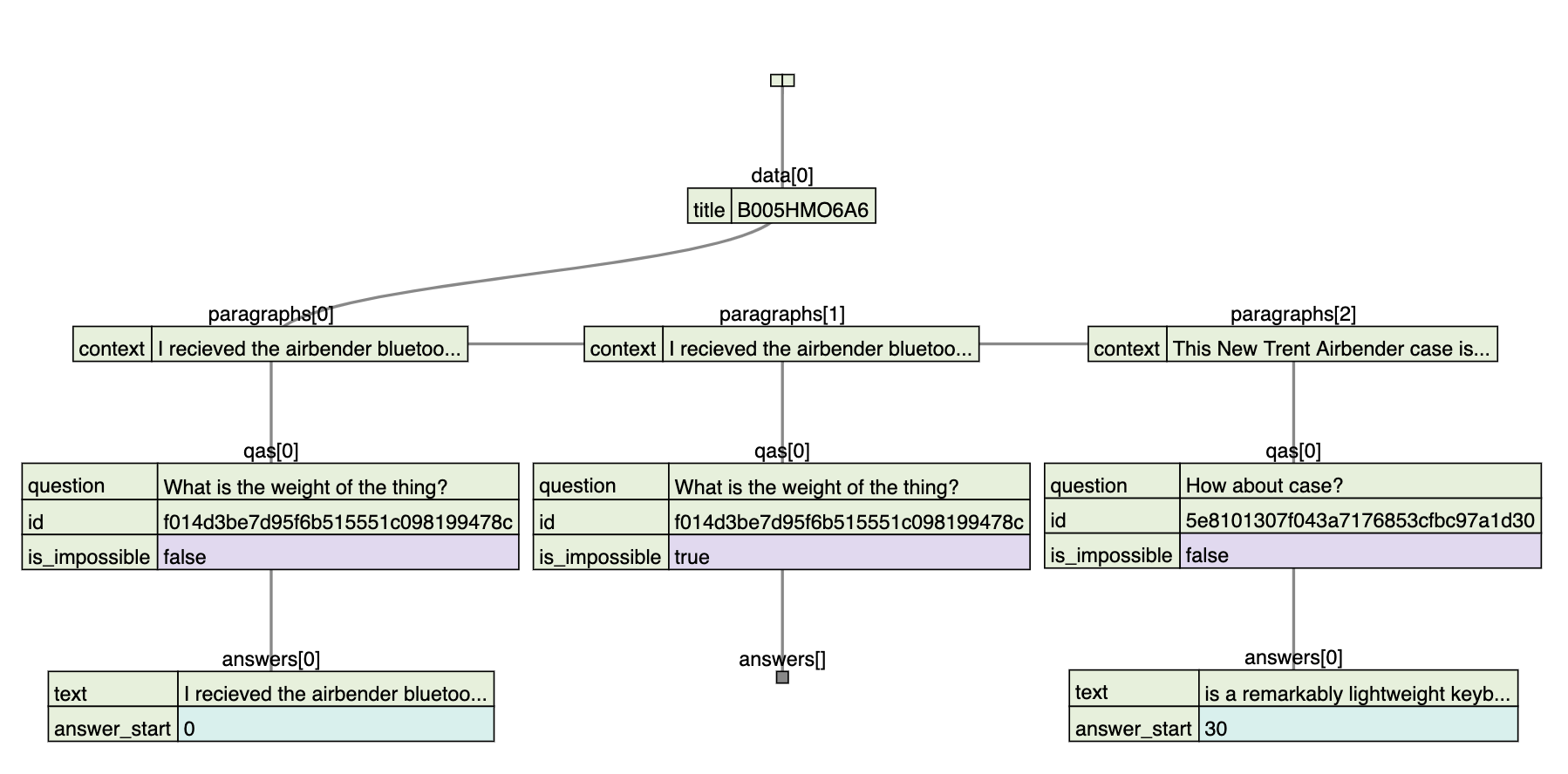
Figure 2-11. Visualization of the SQuAD JSON format.
You can download the pre-processed data from the book’s GitHub repository ADD LINK. Now that we have the splits in the right format, let’s fine-tune our Reader by specifying the location of the train and dev splits, along with the location of where to save the fine-tuned model:
reader.train(data_dir=data,use_gpu=True,n_epochs=1,train_filename=f"{category}-train.json",dev_filename=f"{category}-dev.json",batch_size=16,evaluate_every=500,save_dir="models/haystack/minilm-uncased-squad2-subjqa")
With the Reader fine-tuned, let’s now compare it’s performance on the test set against our baseline model:
reader_eval["Fine-tune on SQuAD + SubjQA"]=evaluate_reader(reader)
plot_reader_eval(reader_eval)

Wow, domain adaptation has increased our EM score by a factor of six and
more than doubled the FARMReader:
minilm_ckpt="microsoft/MiniLM-L12-H384-uncased"minilm_reader=FARMReader(model_name_or_path=minilm_ckpt,progress_bar=False,max_seq_len=max_seq_length,doc_stride=doc_stride,return_no_answer=True)
Next we fine-tune for one epoch:
minilm_reader.train(data_dir=data,use_gpu=True,n_epochs=1,train_filename=f"{category}-train.json",dev_filename=f"{category}-dev.json",batch_size=16,evaluate_every=500,save_dir="models/haystack/minilm-uncased-subjqa")
and include the evaluation on the test set:
reader_eval["Fine-tune on SubjQA"]=evaluate_reader(minilm_reader)
plot_reader_eval(reader_eval)

We can see that fine-tuning the language model directly on SubjQA performs a considerably worse that the model fine-tuned on SQuAD and SubjQA.
Warning
When dealing with small datasets, it is best practice to use cross-validation when evaluating transformers as they can be prone to overfitting. You can find an example for how to perform cross-validation with SQuAD-formatted datasets in the FARM repository.
Evaluating the Whole QA Pipeline
Now that we’ve seen how to evaluate the Reader and Retriever
components individually, let’s tie them together to measure
the overall performance of our pipeline. To do so, we’ll
need to augment our Retriever pipeline with nodes for the Reader and its
evaluation. We’ve seen that we get almost perfect recall at
# Initialize Retriever pipelinepipe=EvalRetrieverPipeline(es_retriever)# Add nodes for Readereval_reader=EvalReader()pipe.pipeline.add_node(component=reader,name="QAReader",inputs=["EvalRetriever"])pipe.pipeline.add_node(component=eval_reader,name="EvalReader",inputs=["QAReader"])# Evaluate!run_pipeline(pipe)# Extract metrics from Readerreader_eval["QA Pipeline (top-1)"]={k:vfork,vineval_reader.__dict__.items()ifkin["top_1_em","top_1_f1"]}reader_eval["QA Pipeline (top-3)"]={k.replace("k","1"):vfork,vineval_reader.__dict__.items()ifkin["top_k_em","top_k_f1"]}
We can then compare the top-1 and top-3

Figure 2-12. Comparison of EM and F1 scores for the Reader against the whole QA pipeline
From this plot we can see the effect that the Retriever has on the overall performance. In particular, there is an overall degradation of performance compared to matching the question-context pairs as is done in the SQuAD-style evaluation. This can be circumvented by increasing the number of possible answers that the Reader is allowed to predict. Until now we have only extracted answer spans from the context but in general it could be that bits and pieces of the answer are scattered throughout the document and we would like our model to synthesize these fragments into a single, coherent answer. Let’s have a look how we can use generative QA to succeed at this task.
Going Beyond Extractive QA
One interesting alternative to extracting answers as spans of text in a document is to generate them with a pretrained language model. This approach is often referred to as abstractive or generative QA and has the potential to produce better phrased answers that synthesize evidence across multiple passages. Although less mature than extractive QA, this is a fast-moving field of research, so chances are that these approaches will be widely adopted in industry by the time you are reading this! In this section we’ll briefly touch the current state-of-the-art: Retrieval Augmented Generation (RAG).14
Retrieval Augmented Generation
RAG extends the classic Retriever-Reader architecture that we’ve seen in this chapter by swapping the Reader for a Generator and using DPR as the Retriever. The Generator is a pretrained sequence-to-sequence transformer like T5 or BART which receives latent vectors of documents from DPR and then iteratively generates an answer based on the query and these documents. Since DPR and the Generator are differentiable, the whole process can be fine-tuned end-to-end as illustrated in Figure 2-13. You can find an interactive demo of RAG on the Hugging Face website.
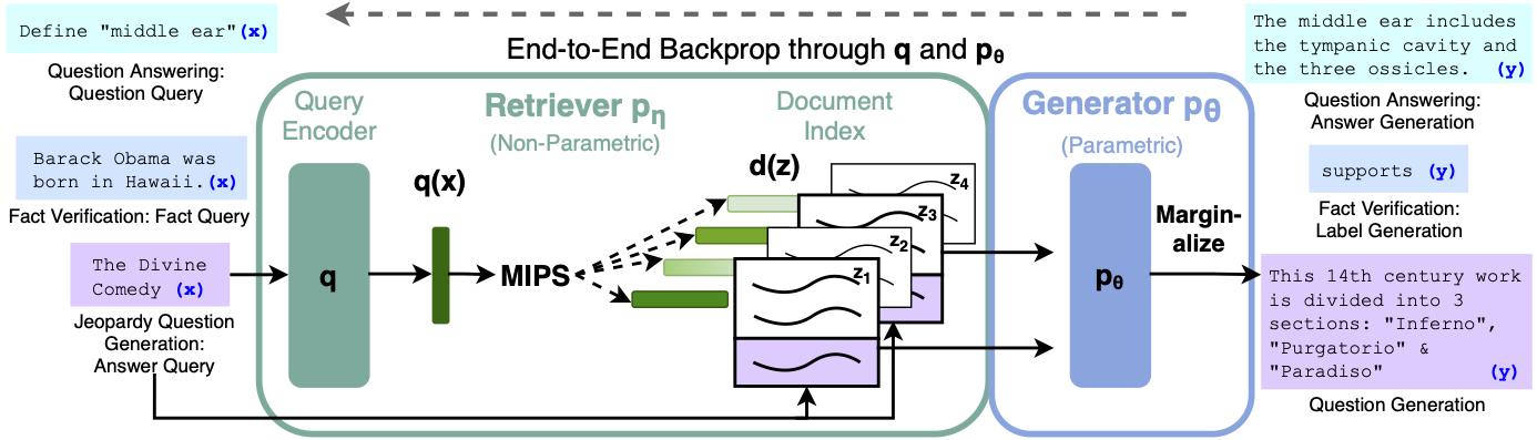
Figure 2-13. The RAG architecture for fine-tuning a Retriever and Generator end-to-end (courtesy of Ethan Perez).
To show RAG in action, we’ll use the DPRetriever from
earlier so we just need to instantiate a Generator. There are two types
of RAG models to choose from:
- RAG-Sequence
-
Uses the same retrieved document to generate the complete answer. In particular, the top-
- RAG-Token
-
Can use a different document to generate each token in the answer. This allows the Generator to synthesize evidence from multiple documents.
Since RAG-Token models tend to perfom better than RAG-Sequence ones,
we’ll use the token model that was fine-tuned on NQ as our
Generator. Instantiating a Generator in Haystack is similar to the
Reader, but instead of specifying the max_seq_length and doc_stride
parameters for a sliding window over the contexts, we specify
hyperparameters that control the text generation:
fromhaystack.generator.transformersimportRAGeneratorgenerator=RAGenerator(model_name_or_path="facebook/rag-token-nq",max_length=300,min_length=50,embed_title=False,num_beams=5)
Here max_length and min_length control the length of the generated
answers, while num_beams specifies the number of beams to use in beam
search (text generation is covered at length in
Chapter 6). As we did with the DPR Retriever, we
don’t embed the document titles since our corpus is always
filtered per product ID.
The next thing to do it tie together the Retriever and Generator using
Haystack’s GenerativeQAPipeline:
fromhaystack.pipelineimportGenerativeQAPipelinepipe=GenerativeQAPipeline(generator=generator,retriever=dpr_retriever)
Note
In RAG, both the query encoder and the generator are trained end-to-end, while the context encoder is frozen. In Haystack, the GenerativeQAPipeline uses the query encoder from RAGenerator and the context encoder from DensePassageRetriever.
Let’s now give RAG a spin by feeding some queries about the Amazon Fire tablet from before. To simplify the querying, let’s write a simple function that takes query and prints out the top answers:
defgenerate_answers(query,top_k_generator=3):preds=pipe.run(query=query,top_k_generator=top_k_generator,top_k_retriever=5,filters={"item_id":["B0074BW614"]})(f"Question: {preds['query']}","")foridxinrange(top_k_generator):(f"Answer {idx+1}: {preds['answers'][idx]['answer']}")
Okay, now we’re ready to give it a test:
generate_answers(query)
Question: Is it good for reading?

Answer 1:  Kindle fire
Answer 2: Kindle fire
Answer 3:  e-reader
Hmm, this result it a bit disappointing and suggests that the subjective nature of the question is confusing the Generator. Let’s try with something a bit more factual:
generate_answers("What is the main drawback?")
Question: What is the main drawback?

Answer 1:  the price
Answer 2:  the power cord connection
Answer 3:  the cost
Okay, this is more sensible! To get better results we could fine-tune RAG end-to-end on SubjQA, and if you’re interested in exploring this there are scripts in the Transformers repository to help you get started.
Conclusion
Well, that was a whirlwind tour of QA and you probably have many more questions that you’d like answered (pun intended!). We have discussed two approaches to QA (extractive and generative), and examined two different retrieval algorithms (BM25 and DPR). Along the way, we saw that domain adaptation can be a simple technique to boost the performance of our QA system by a significant margin, and we looked at a few of the most common metrics that are used for evaluating such systems. Although we focused on closed-domain QA (i.e. a single domain of electronic products), the techniques in this chapter can easily be generalized to the open-domain case and we recommend reading Cloudera’s excellent Fast Forward QA series to see what’s involved.
Deploying QA systems in the wild can be a tricky business to get right, and our experience is that a significant part of the value comes from first providing end-users with useful search capabilities, followed by an extractive component. In this respect, the Reader can be used in novel ways beyond answering on-demand user queries. For example, Grid Dynamics were able to use their Reader to automatically extract a set of pros and cons for each product in their client’s catalogue. Similarly, they show that a Reader can also be used to extract named entities in a zero-shot fashion by creating queries like “What kind of camera?”. Given its infancy and subtle fail-modes, we recommend exploring answering generation only once the other two approaches have been exhausted. This “hierarchy of needs” for tackling QA problems is illustrated in Figure 2-14.
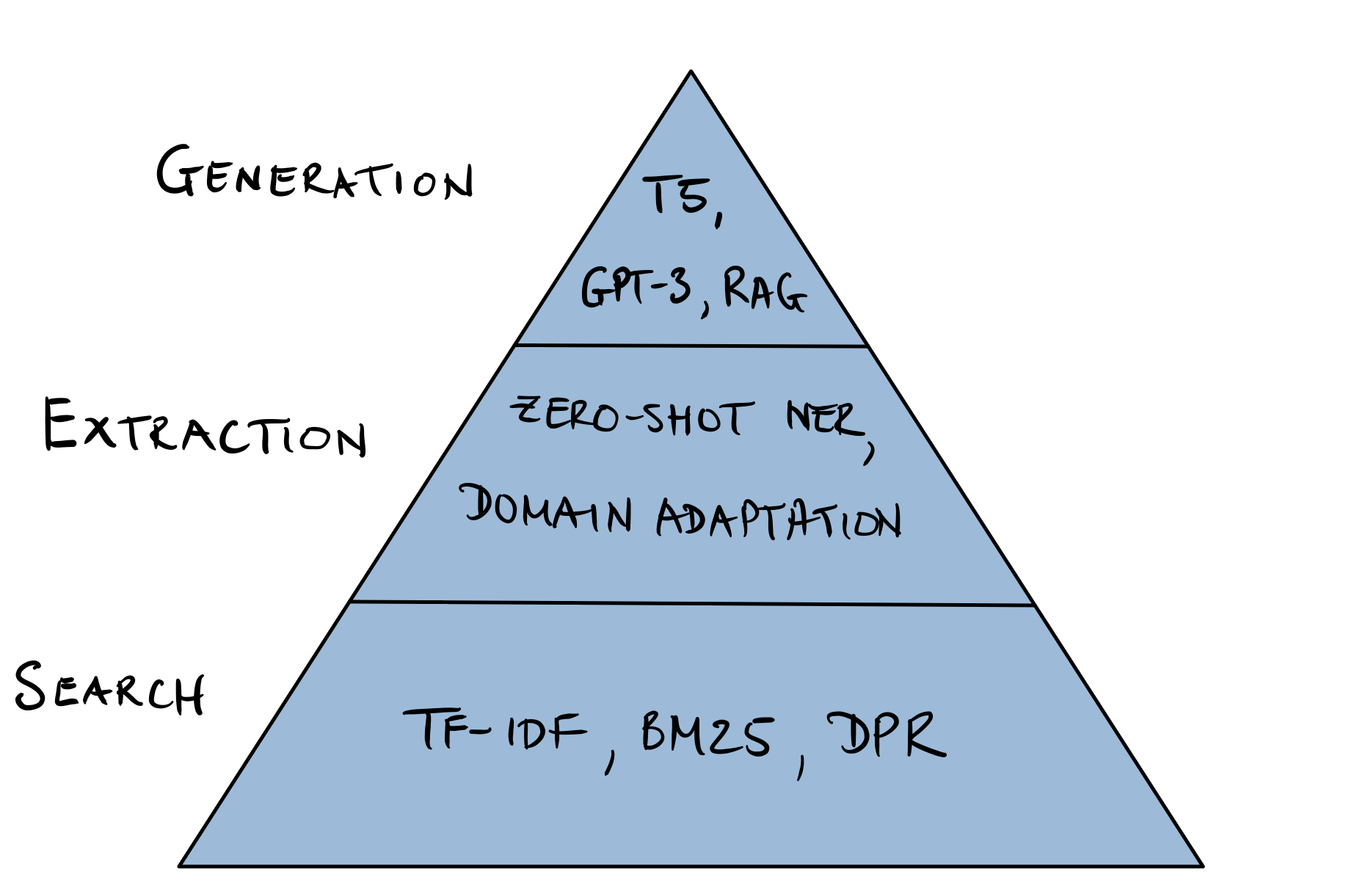
Figure 2-14. The QA hierarchy of needs.
Looking towards the future, one exciting research area to keep an eye on is multimodal QA which involves QA over multiple modalities like text, tables, and images. As described in the MultiModalQA benchmark15, such systems can potentially enable users to answer complex questions like “When was the famous painting with two touching fingers completed?” which integrate information across different modalities. Another area with practical business applications is QA over a knowledge graph, where the nodes of the graph correspond to real-world entities and their relations are defined by the edges. By encoding factoids as (subject, predicate, object) triples, one can use the graph to answer questions about one of the missing elements. You can find an example that combines transformers with knowledge graphs in the Haystack tutorials. One last promising direction is “automatic question generation” as a way to do some form of unsupervised/weakly supervized training from unlabelled data or data augmentation. Two recent examples of papers on this include the Probably Answered Questions (PAQ) benchmark16 and synthetic data augmentation17 for cross-lingual settings.
In this chapter we’ve seen that in order to successfully use QA models in real world use-cases we need to apply a few tricks such as a fast retrieval pipeline to make predictions in near real-time. Still, applying a QA model to a handful of preselected documents can take a couple of seconds on production hardware. Although this does not sound like much imagine how different your experience would be if you had to wait a few seconds to get the results of your Google search. A few seconds of wait time can decide the fate of your transformer powered application and in the next chapter we have a look at a few methods to accelerate the model predictions further.
1 In this particular case, providing no answer at all may actually be the right choice, since the answer depends on when the question is asked and concerns a global pandemic where having accurate health information is essential.
2 SUBJQA: A Dataset for Subjectivity and Review Comprehension, J. Bjerva et al. (2020)
3 As we’ll soon see, there are also unanswerable questions that are designed to produce more robust reading comprehension models.
4 SQuAD: 100,000+ Questions for Machine Comprehension of Text, P. Rajpurkar et al. (2016)
5 MINILM: Deep Self-Attention Distillation for Task-Agnostic Compression of Pre-Trained Transformers, W. Wang et al (2020)
6 Note that the token_type_ids are not present in all transformer models. In the case of BERT-like models such as MiniLM, the token_type_ids are also used during pretraining to incorporate the next-sentence prediction task.
7 See Chapter 1 for details on how these hidden states can be extracted.
8 Know What You Don’t Know: Unanswerable Questions for SQuAD, P. Rajpurkar, R. Jia, and P. Liang (2018)
9 Natural Questions: a Benchmark for Question Answering Research, T. Kwiatkowski et al (2019)
10 The guide also provides installation instructions for mac OS and Windows.
11 For an in-depth explanation on document scoring with TF-IDF and BM25 see Chapter 23 of Speech and Language Processing, D. Jurafsky and J.H. Martin (2020)
12 Dense Passage Retrieval for Open-Domain Question Answering, V. Karpukhin et al (2020)
13 Learning and Evaluating General Linguistic Intelligence D. Yogatama et al. (2019)
14 Retrieval-Augmented Generation for Knowledge-Intensive NLP Tasks, P. Lewis et al (2020)
15 MultiModalQA: Complex question answering over text, tables and images, A. Talmor et al (2021)
16 PAQ: 65 Million Probably-Asked Questions and What You Can Do With Them, P. Lewis et al (2021).
17 Synthetic Data Augmentation for Zero-Shot Cross-Lingual Question Answering, A. Riabi et al (2020).