Chapter 3. Using Data from Your Network

In Chapter 2, “Data for Network Automation,” you learned about data types and data models, as well as common methods to gather data from your network infrastructure. After you have stored your network data, what do you do with it? Are you currently storing any of your network’s data (logs, metrics, configurations)? If so, which data? What for?

You typically store data in order to find insights in it and to comply with regulatory requirements. An insight, in this sense, can be any useful information or action.

This chapter helps you understand how to use the collected data from your network and derive value from it. In the context of enterprise networks, this chapter covers the following topics:

• Data preparation techniques

• Data visualization techniques

• Network insights

At the end of this chapter are some real case studies that are meant to inspire you to implement automation solutions in your own network.

Data Preparation

Data comes in various formats, such as XML, JSON, and flow logs (refer to Chapter 2). It would be nice if we could gather bread from a field, but we must gather wheat and process it into bread. Similarly, after we gather data from a variety of devices, we need to prepare it. When you have a heterogeneous network, even if you are gathering the same type of data from different places, it may come in different formats (for example, NetFlow on a Cisco device and IPFIX on an HPE device). Data preparation involves tailoring gathered data to your needs.

There are a number of data preparation methods. Data preparation can involve simple actions such as normalizing the date format to a common one as well as more complex actions such as aggregating different data points. The following sections discuss some popular data preparation methods that you should be familiar with.

Parsing

Most of the times when you gather data, it does not come exactly as you need it. It may be in different units, it may be too verbose, or you might want to split it in order to store different components separately in a database. In such cases, you can use parsing techniques.

There are many ways you can parse data, including the following:

• Type formatting: You might want to change the type, such as changing seconds to minutes.

• Splitting into parts: You might want to divide a bigger piece of information into smaller pieces, such as changing a sentence into words.

• Tokenizing: You might want to transform a data field into something less sensitive, such as when you store payment information.

You can parse data before storage or when consuming it from storage. There is really no preferred way, and the best method depends on the architecture and storage capabilities. For example, if you store raw data, it is possible that afterward, you might parse it in different ways for different uses. If you store raw data, you have many options for how to work with that data later; however, it will occupy more storage space, and those different uses may never occur. If you choose to parse data and then store it, you limit what you store, which saves space. However, you might discard or filter a field that you may later need for a new use case.

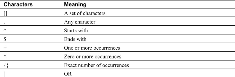
Regular expressions (regex) play a big part in parsing. Regex, which are used to find patterns in text, exist in most automation tools and programming languages (for example, Python, Java). It is important to note that, regardless of the tool or programing language used, the regex are the same. Regex can match specific characters, wildcards, and sequences. They are not predefined; you write your own to suit your need, as long as you use the appropriate regex syntax. Table 3-1 describes the regex special characters.

Table 3-1 Regex Special Characters

Table 3-2 describes a number of regex meta characters; although this is not a complete list, these are the most commonly used meta characters.

Table 3-2 Regex Meta Characters

Example 3-1 shows how to use regex to find the IP address of an interface.

Example 3-1 Using Regex to Identify an IPv4 Address

Given the configuration:
interface Loopback0
description underlay
ip address 10.0.0.1 255.255.255.0

Regex expression:
(?:[0-9]{1,3}.){3}[0-9]{1,3}

Result:
["10.0.0.1", "255.255.255.0"]

Example 3-1 shows a simplex regex that matches on three blocks of characters that range from 0 to 999 and have a trailing dot, followed by a final block of characters ranging from 0 to 999. The result in this configuration is two entries that correspond to the IP address and the mask of the Loopback0 interface.

IP addresses are octets, with each unit consisting of 8 bits ranging from 0 to 255. As an exercise, improve the regex in Example 3-1 to match only the specific 0 to 255 range in each IP octet. To try it out, find one of the many websites that let you insert text and a regex and then show you the resulting match.

You can also use a number of tools, such as Python and Ansible, to parse data. Example 3-2 shows how to use Ansible for parsing. Firstly, it lists all the network interfaces available in a Mac Book laptop, using the code in the file all_interfaces.yml. Next, it uses the regex ˆen to display only interfaces prefixed with en. This is the code in en_only.yml.

Example 3-2 Using Ansible to Parse Device Facts

$ cat all_interfaces.yml
---
- hosts: all
  tasks:
    - name: print interfaces
      debug:
        msg: "{{ ansible_interfaces }}"
$ ansible-playbook -c local -i 'localhost,' all_interfaces.yml
PLAY [all] *********************************************************************

TASK [Gathering Facts]
*********************************************************************
ok: [localhost]

TASK [print interfaces]
*********************************************************************
ok: [localhost] => {
    "msg": [
        "awdl0",
        "bridge0",
        "en0",
        "en1",
        "en2",
        "en3",
        "en4",
        "en5",
        "gif0",
        "llw0",
        "lo0",
        "p2p0",
        "stf0",
        "utun0",
        "utun1”
    ]
}
PLAY RECAP *********************************************************************
localhost                  : ok=2    changed=0    unreachable=0    failed=0    skipped=0
rescued=0    ignored=0

$ cat en_only.yml
---
- hosts: all
  tasks:
    - name: print interfaces
      debug:
        msg: "{{ ansible_interfaces | select('match', '^en') | list }}"

$ ansible-playbook -c local -i 'localhost,' en_only.yml

PLAY [all] *********************************************************************

TASK [Gathering Facts]
*********************************************************************
ok: [localhost]

TASK [print interfaces]
*********************************************************************
ok: [localhost] => {
    "msg": [
        "en0",
        "en1",
        "en2",
        "en3",
        "en4",
        "en5”
    ]
}

PLAY RECAP *********************************************************************
localhost                  : ok=2    changed=0    unreachable=0    failed=0    skipped=0
rescued=0    ignored=0

What if you need to apply modifications to interface names, such as replacing en with Ethernet? In such a case, you can apply mapping functions or regex, as shown with Ansible in Example 3-3.

Example 3-3 Using Ansible to Parse and Alter Interface Names

$ cat replace_ints.yml
---
- hosts: all
  tasks:
    - name: print interfaces
      debug:
        msg: "{{ ansible_interfaces | regex_replace('en', 'Ethernet') }}"

$ ansible-playbook -c local -i 'localhost,' replace_ints.yml

PLAY [all] *********************************************************************

TASK [Gathering Facts]
*********************************************************************
ok: [localhost]

TASK [print interfaces]
*********************************************************************
ok: [localhost] => {
    "msg": [
        "awdl0",
        "bridge0",
        "Ethernet0",
        "Ethernet1",
        "Ethernet2",
        "Ethernet3",
        "Ethernet4",
        "Ethernet5",
        "gif0",
        "llw0",
        "lo0",
        "p2p0",
        "stf0",
        "utun0",
        "utun1"
    ]
}

PLAY RECAP *********************************************************************
localhost                  : ok=2    changed=0    unreachable=0    failed=0    skipped=0
rescued=0    ignored=0

Another technique that can be considered parsing is enhancing data with other fields. Although this is typically done before storage and not before usage, consider that sometimes the data you gather might not have all the information you need to derive insights. For example, flow data might have SRC IP, DST IP, SRC port, and DST port information but no date. If you store that data as is, you might be able to get insights from it on the events but not when they happened. Something you could consider doing in this scenario is appending or prepending the current date to each flow and then storing the flow data.

As in the previous example, there are many use cases where adding extra data fields can be helpful—such as with sensor data that does include have sensor location or system logs that do not have a field indicating when maintenance windows take place. Adding extra data fields is a commonly used technique when you know you will need something more than just the available exported data.

Example 3-4 enhances the previous Ansible code (refer to Example 3-3) by listing the available interfaces along with the time the data was collected.

Example 3-4 Using Ansible to List Interfaces and Record Specific Times

$ cat fieldadd.yml
---
- hosts: all
  tasks:
    - name: print interfaces
      debug:
        msg: "{{ ansible_date_time.date + ansible_interfaces | regex_replace('en',
'Ethernet') }} "
$ ansible-playbook -c local -i 'localhost,' fieldadd.yml

PLAY [all] *********************************************************************

TASK [Gathering Facts]
*********************************************************************
ok: [localhost]

TASK [print interfaces]
*********************************************************************
ok: [localhost] => {
    "msg": "2021-01-22['awdl0', 'bridge0', 'Ethernet0', 'Ethernet1', 'Ethernet2',
'Ethernet3', 'Ethernet4', 'Ethernet5', 'gif0', 'llw0', 'lo0', 'p2p0', 'stf0', 'utun0',
'utun1'] "
}

PLAY RECAP *********************************************************************
localhost                  : ok=2    changed=0    unreachable=0    failed=0    skipped=0
rescued=0    ignored=0

As part of parsing, you might choose to ignore some data. That is, you might simply drop it instead of storing or using it. Why would you do this? Well, you might know that some of the events that are taking place taint your data. For example, say that during a maintenance window you must physically replace a switch. If you have two redundant switches in your architecture, while you are replacing one of them, all your traffic is going through the other one. The data collected will reflect this, but it is not a normal scenario, and you know why it is happening. In such scenarios, ignoring data points can be useful, especially to prevent outliers on later analysis.

So far, we have mostly looked at examples of using Ansible to parse data. However, as mentioned earlier, you can use a variety of tools for parsing.

Something to keep in mind is that the difficulty of parsing data is tightly coupled with its format. Regex are typically used for text parsing, and text is the most challenging type of data to parse. Chapter 2 mentions that XQuery and XPath can help you navigate XML documents. This should give you the idea that different techniques can be used with different types of data. Chapter 2’s message regarding replacing the obsolete CLI access with NETCONF, RESTCONF, and APIs will become clearer when you need to parse gathered data. Examples 3-5 and 3-6 show how you can parse the same information gathered in different formats from the same device.

Example 3-5 Using Ansible with RESTCONF to Retrieve an Interface Description

$ cat interface_description.yml
---
- name: Using RESTCONF to retrieve interface description
  hosts: all
  connection: httpapi

  vars:
    ansible_connection: httpapi
    ansible_httpapi_port: 443
    ansible_httpapi_use_ssl: yes
    ansible_network_os: restconf
    ansible_user: cisco
    ansible_httpapi_password: cisco123

  tasks:
    - name: Retrieve interface configuration
      restconf_get:
        content: config
        output: json
        path: /data/ietf-interfaces:interfaces/interface=GigabitEthernet1%2F0%2F13
      register: cat9k_rest_config

    - name: Print all interface configuration
      debug: var=cat9k_rest_config

    - name: Print interface description
      debug: var=cat9k_rest_config['response']['ietf-
interfaces:interface']['description']

$ ansible-playbook -i '10.201.23.176,' interface_description.yml

PLAY [Using RESTCONF to retrieve interface description]
*********************************************************************
TASK [Retrieve interface configuration]
*********************************************************************
ok: [10.201.23.176]

TASK [Print all interface configuration] ***************************************
ok: [10.201.23.176] => {
    "cat9k_rest_config": {
        "ansible_facts": {
            "discovered_interpreter_python": "/usr/bin/python"
        },
        "changed": false,
        "failed": false,
        "response": {
            "ietf-interfaces:interface": {
                "description": "New description”,
                "enabled": true,
                "ietf-ip:ipv4": {
                    "address": [
                        {
                            "ip": "172.31.63.164",
                            "netmask": "255.255.255.254"
                        }
                    ]
                },
                "ietf-ip:ipv6": {},
                "name": "GigabitEthernet1/0/13",
                "type": "iana-if-type:ethernetCsmacd"
            }
        },
        "warnings": []
    }
}

TASK [Print interface description] *********************************************
ok: [10.201.23.176] => {
    "cat9k_rest_config['response']['ietf-interfaces:interface']['description']": "New
description”
}

PLAY RECAP *********************************************************************
10.201.23.176              : ok=3    changed=0    unreachable=0    failed=0    skipped=0
rescued=0    ignored=0

In Example 3-5, you can see that when using a RESTCONF module, you receive the interface information in JSON format. Using Ansible, you can navigate through the JSON syntax by using the square bracket syntax. It is quite simple to access the interface description, and if you needed to access some other field, such as the IP address field, you would need to make only a minimal change:

debug: var=cat9k_rest_config['response']['ietf-interfaces:interface']['ietf-ip:ipv4']

Example 3-6 achieves the same outcome by using a CLI module and regex.

Example 3-6 Using Ansible with SSH and Regex to Retrieve an Interface Description

$ cat interface_description.yml
---
- name: Retrieve interface description
  hosts: all
  gather_facts: no

  vars:
    ansible_user: cisco
    ansible_password: cisco123
    interface_description_regexp: "description [\w+ *]*”

  tasks:
    - name: run show run on device
      cisco.ios.ios_command:
        commands: show run interface GigabitEthernet1/0/13
      register: cat9k_cli_config

    - name: Print all interface configuration
      debug: var=cat9k_cli_config

    - name: Scan interface configuration for description
      set_fact:
        interface_description: "{{ cat9k_cli_config.stdout[0] |
regex_findall(interface_description_regexp, multiline=True) }}”

    - name: Print interface description
      debug: var=interface_description

$ ansible-playbook -i '10.201.23.176,' interface_description.yml
PLAY [Retrieve interface description]
********************************************************************

TASK [run show run on device]
*********************************************************************
ok: [10.201.23.176]

TASK [Print all interface configuration]
*********************************************************************
ok: [10.201.23.176] => {
    "cat9k_cli_config": {
        "ansible_facts": {
            "discovered_interpreter_python": "/usr/bin/python"
        },
        "changed": false,
        "deprecations": [
            {}
        ],
        "failed": false,
        "stdout": [
            "Building configuration...

Current configuration : 347
bytes
!
interface GigabitEthernet1/0/13
 description New description
 no
switchport
 dampening
 ip address 172.31.63.164 255.255.255.254
 no ip redirects
 ip
pim sparse-mode
 ip router isis 
 load-interval 30
 bfd interval 500 min_rx 500
 multiplier 3
 clns mtu 1400
 isis network point-to-point 
end"
        ],
        "stdout_lines": [
            [
                "Building configuration...",
                "",
                "Current configuration : 347 bytes",
                "!",
                "interface GigabitEthernet1/0/13",
                " description New description",
                " no switchport",
                " dampening",
                ” ip address 172.31.63.165 255.255.255.254 secondary",
                " ip address 172.31.63.164 255.255.255.254",
                " no ip redirects",
                " ip pim sparse-mode",
                ” ip router isis ",
                ” load-interval 30",
                " bfd interval 500 min_rx 500 multiplier 3",
                ” clns mtu 1400",
                " isis network point-to-point ",
                "end"
            ]
        ],
        "warnings": []
    }
}

TASK [Scan interface configuration for description]
*********************************************************************
ok: [10.201.23.176]

TASK [Print interface description]
*********************************************************************
ok: [10.201.23.176] => {
    "interface_description": [
        "description New description”
    ]
}

PLAY RECAP *********************************************************************
10.201.23.176              : ok=4    changed=0    unreachable=0    failed=0    skipped=0
rescued=0    ignored=0

Example 3-6 uses the following regex:

"description [\w+ *]*”

This is a simple regex example, but things start to get complicated when you need to parse several values or complex values. Modifications to the expected values might require building new regex, which can be troublesome.

By now you should be seeing the value of the structured information you saw in Chapter 2.

Aggregation

Data can be aggregated—that is, used in a summarized format—from multiple sources or from a single source. There are multiple reasons you might need to aggregate data, such as when you do not have enough computing power or networking bandwidth to use all the data points or when single data points without the bigger context can lead to incorrect insights.

Let’s look at a networking example focused on the CPU utilization percentage in a router. If you are polling the device for this percentage every second, it is possible that for some reason (such as a traffic burst punted to CPU), it could be at 100%, but then, in the next second, it drops to around 20% and stays there. In this case, if you have an automated system to act on the monitored metric, you will execute a preventive measure that is not needed. Figure 3-1 and 3-2 show exactly this, where a defined threshold for 80% CPU utilization would trigger if you were measuring each data point separately but wouldn’t if you aggregated the data and used the average of the three data points.

Figure 3-1 % CPU Utilization Graph per Time Measure T

Figure 3-2 % CPU Utilization Graph per Aggregated Time Measure T

In the monitoring use case, it is typical to monitor using aggregated results at time intervals (for example, 15 or 30 seconds). If the aggregated result is over a defined CPU utilization threshold, it is a more accurate metric to act on. Tools like Kibana support aggregation natively.

As another example of aggregating data from multiple sources to achieve better insights, consider the following scenario: You have two interfaces connecting the same two devices, and you are monitoring all interfaces for bandwidth utilization. Your monitoring tool has a defined threshold for bandwidth utilization percentage and automatically provisions a new interface if the threshold is reached. For some reason, most of your traffic is taking one of the interfaces, which triggers your monitoring tool’s threshold. However, you still have the other interface bandwidth available. A more accurate aggregated metric would be the combined bandwidth available for the path (an aggregate of the data on both interfaces).

Finally, in some cases, you can aggregate logs with the addition of a quantifier instead of repeated a number of times—although this is often out of your control because many tools either do not support this feature or apply it automatically. This type of aggregation can occur either in the device producing the logs or on the log collector. It can be seen as a compression technique as well (see Example 3-7). This type of aggregation is something to have in mind when analyzing data rather than something that you configure.

Example 3-7 Log Aggregation on Cisco’s NX-OS

Original:
2020 Dec  24 09:34:11 N7009 %VSHD-5-VSHD_SYSLOG_CONFIG_I: Configured from vty by ivpinto on 10.10.10.1@pts/0
2020 Dec  24 09:35:09 N7009 %VSHD-5-VSHD_SYSLOG_CONFIG_I: Configured from vty by ivpinto on 10.10.10.1@pts/0
Aggregated:
2020 Dec  24 09:34:11 N7009 %VSHD-5-VSHD_SYSLOG_CONFIG_I: Configured from vty by ivpinto on 10.10.10.1@pts/0
2020 Dec  24 09:35:09 N7009 last message repeated 1 time

Data Visualization

Humans are very visual. A good visualization can illustrate a condition even if the audience does not have technical knowledge. This is especially helpful for alarming conditions. For example, you do not need to understand that the CPU for a device should not be over 90% if there is a red blinking light over it.

Visualizing data can help you build better network automation solutions or even perceive the need for an automated solution. However, automation solutions can also build data visualization artifacts.

There are a number of tools that can help you visualize data. For example, Chapter 1, “Types of Network Automation,” discusses Kibana, which can be used for log data; Grafana, which can be used for metric data; and Splunk, which can be used for most data types. There are also data visualization tools specific for NetFlow or IPFIX data; for example, Cisco’s Tetration. This type of flow data is typically exported to specialized tools to allow you to visualize who the endpoints are talking to, what protocols they are using, and what ports they are using.

Say that you want to visualize the CPU utilization of routers. The best data gathering method in this scenario would be model-driven telemetry (but if telemetry is not available, SNMP can also work), and Grafana would be a good visualization choice. Grafana integrates with all kinds of databases, but for this type of time-series data, InfluxDB is a good fit. The configuration steps would be as follows:

Step 1. Configure a telemetry subscription in the router.

Step 2. Configure a telemetry server (for example, Telegraf) to listen in.

Step 3. Store the data in a database (for example, InfluxDB).

Step 4. Configure Grafana’s data source as the database table.

The resulting visualization might look like the one in Figure 3-3, where you can see the millicores on the vertical axis and the time on the horizontal axis.

Figure 3-3 Grafana Displaying a Router CPU Utilization Graph per Minute

This type of data visualization could alert you to the need for an automated solution to combat CPU spikes, for example, if they are occurring frequently and impacting service. Many times, it is difficult to perceive a need until you see data represented in a visual format.

Although data visualization is a discipline on its own and we only touch on a very small part of it, there are a couple things to have in mind when creating visualizations. For one thing, you should choose metrics that clearly represent the underlying status. For example, for CPU utilization, typically the percentage is shown and not cores or threads. This is because interpreting a percentage is much easier than knowing how many cores are available on a specific device and contrasting that information with the devices being used. On the other hand, when we are looking at memory, most of the time we represent it with a storage metric (such as GB or MB) rather than a percentage. Consider that 10% of memory left can mean a lot in a server with 100 TB but very little in a server with 1 TB; therefore, representing this metric as 10 TB left or 100 GB left would be more illustrative.

Choosing the right metric scale can be challenging. Table 3-3 illustrates commonly used scales for enterprise network component visualizations.

Table 3-3 Data Visualization Scales

Another important decision is visualization type. There are many commonly used visualizations. The following types are commonly used in networking:

• Line charts

• Stat panels/gauges

• Bar charts

Your choice of visualization will mostly come down to two answers:

• Are you trying to compare several things?

• Do you need historical context?

The answer to the first question indicates whether you need multiple- or single-line visualizations. For example, if you want to visualize the memory usage of all components within a system, you could plot it as shown in Figure 3-4. This line chart with multiple lines would allow you to compare the components and get a broader perspective. In this figure, you can see that the app-hosting application is consuming more than twice as much memory as any other running application.

Figure 3-4 Virtual Memory Utilization Graph of All Components in a Container

If you simply want to see the memory usage for a single component, such as a router or an application running on a system, you do not need to pollute your visualization with unneeded information that would cause confusion without adding value. In this case, a single-line chart like the one in Figure 3-5 would suffice.

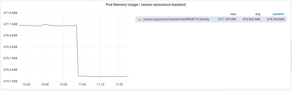
Figure 3-5 Virtual Memory Utilization Graph of Sensor Assurance Application

Both Figures 3-4 and 3-5 give you a chronological view of the metric being measured. If you do not need historical context, and you just want to know the status at the exact moment, you can use panels or bar charts instead. For example, Figure 3-6 shows a point-in-time view of the Figure 3-4 metrics.

Figure 3-6 Current Virtual Memory Utilization Bar Chart of All Components in a Container

When you do not need a chronological understanding of a metric and you have a single component to represent, the most commonly used visualization is a gauge or a stat panel. Figure 3-7 shows a point-in-time view of the Figure 3-5 metric.

Figure 3-7 Gauge Representation of the Current Virtual Memory Utilization of Sensor Assurance Application

A way to further enhance visualization is to use color. You can’t replace good visualization metrics and types with color. However, color can enhance good visualization metrics and types. Color thresholds in visualizations can enable quicker insights. For example, by defining 80% memory utilization or higher as red, 60% to 79% utilization as yellow, and 59% or less as green, a visualization can help an operator get a feeling for the overall status of a system with a simple glance at a dashboard.

In some cases, you might want to automate a data visualization instead of using a prebuilt tool. This might be necessary if your use case is atypical, and market tools do not fulfill it. For example, say that a customer has an ever-growing and ever-changing network. The network engineers add devices, move devices across branches, and remove devices every day. The engineering team wants to have an updated view of the topology when requested. The team is not aware of any tool on the market that can achieve this business need, so it decides to build a tool from scratch. The team uses Python to build an automated solution hosted on a central station and that consists of a tool that collects CDP neighbor data from devices, cross-references the data between all devices, and uses the result to construct network diagrams. This tool can be run at any time to get an updated view of the network topology.

Data Insights

An insight, as mentioned earlier, is knowledge gained from analyzing information. The goal of gathering data is to derive insights. How do you get insights from your data? In two steps:

Step 1. You need to build a knowledge base. Knowing what is expected behavior and what is erroneous behavior is critical when it comes to understanding data. This is where you, the expert, play a role. You define what is good and what is bad. In addition, new techniques can use the data itself to map what is expected behavior and what is not. We touch on these techniques later in this section.

Step 2. You apply the knowledge base to the data—hopefully automatically, as this is a network automation book.

As an example of this two-step process, say that you define that if a device is running at 99% CPU utilization, this is a bad sign (step 1). By monitoring your devices and gathering CPU utilization data, you identify that a device is running at 100% utilization (step 2) and replace it. The data insight here is that a device was not working as expected.

Alarms

Raising an alarm is an action on the insight (in this case, the insight that it’s necessary to raise the alarm). You can trigger alarms based on different types of data, such as log data or metrics.

You can use multiple tools to generate alarms (refer to Chapter 1); the important parameter is what to alarm on. For example, say that you are gathering metrics from your network using telemetry, and among these metrics is memory utilization. What value for memory utilization should raise an alarm? There is no universal answer; it depends on the type of system and the load it processes. For some systems, running on 90% memory utilization is common; for others, 90% would indicate a problem. Defining the alarm value is referred to as defining a threshold. Most of the time, you use your experience to come up with a value.

You can also define a threshold without having to choose a critical value. This technique, called baselining, determines expected behavior based on historical data.

A very simple baselining technique could be using the average from a specific time frame. However, there are also very complex techniques, such as using neural networks. Some tools (for example, Cisco’s DNA Center) have incorporated baselining modules that help you set up thresholds.

If you are already using Grafana, creating an alarm is very simple. By editing the Figure 3-4 dashboard as shown in Figure 3-8, you can define the alarm metric. You can use simple metrics such as going over a determined value, or calculated metrics such as the average over a predefined time. Figure 3-8 shows a monitoring graph of disk I/O operations on several services; it is set to alarm if the value reaches 55 MBs.

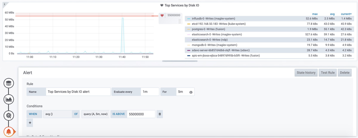
Figure 3-8 Setting Up a Grafana Alarm for 55 MBs Disk I/O

Tools like Kibana also allow you to set up alerts based on log data. For example, Figure 3-9 shows the setup of an alarm based on receiving more than 75 Syslog messages from a database with the error severity in the past 5 minutes.

Figure 3-9 Setting Up a Kibana Alarm for Syslog Data

In addition to acting as alerts for humans, alarms can be automation triggers; that is, they can trigger automated preventive or corrective actions. Consider the earlier scenario of abnormally high CPU utilization percentage. In this case, a possible alarm could be a webhook that triggers an Ansible playbook to clean up known CPU-consuming processes.

Figure 3-10 illustrates an attacker sending CPU punted packets to a router, which leads to a spike in CPU usage. This router is configured to send telemetry data to Telegraf, which stores it in an InfluxDB database. As Grafana ingests this data, it notices the unusual metric and triggers a configured alarm that uses an Ansible Tower webhook to run a playbook and configure an ACL that will drop packets from the attacker, mitigating the effects of the attack.

Figure 3-10 Automated Resolution Triggered by Webhook

Typically, deploying a combination of automated action and human notification is the best choice. Multiple targets are possible when you set up an alarm to alert humans, such as email, SMS, dashboards, and chatbots (for example, Slack or Webex Teams).

In summary, you can use an alarm to trigger actions based on a state or an event. These actions can be automated or can require manual intervention. The way you set up alarms and the actions available on alarms are tightly coupled with the tools you use in your environment. Grafana and Kibana are widely used in the industry, and others are available as well, including as Splunk, SolarWinds, and Cisco’s DNA Center.

Configuration Drift

In Chapter 1, we touched on is the topic of configuration drift. If you have worked in networking, you know it happens. Very few companies have enough controls in place to completely prevent it, especially if they have long-running networks that have been in place more than 5 years. So, how do you address drift?

You can monitor device configurations and compare them to known good ones (templates). This tells you whether configuration drift has occurred. If it has, you can either replace the device configuration with the template or the other way around. The decision you make depends on what is changed.

You can apply templates manually, but if your network has a couple hundred or even thousands of devices, it will quickly become a burden. Ansible can help with this task, as shown in Example 3-8.

Example 3-8 Using Ansible to Identify Configuration Differences in a Switch

$ cat config_dif.yml
---
- hosts: all
  gather_facts: no
  tasks:
    - name: diff against the startup config
      cisco.ios.ios_config:
        diff_against: intended
        intended_config: "{{ lookup('file', 'template.txt') }}”

$ cat inv.yaml
all:
  hosts:
    switch_1:
      ansible_host: "10.10.10.1"
      ansible_network_os: cisco.ios.ios
  vars:
    ansible_connection: ansible.netcommon.network_cli
    ansible_user: "cisco"
    ansible_password: "C!sc0123"

$ ansible-playbook -i inv.yaml config_dif.yml –diff
PLAY [all] *********************************************************************

TASK [diff against the startup config]
*********************************************************************
ok: [switch_1]

PLAY RECAP *********************************************************************
switch_1                   : ok=1    changed=0    unreachable=0    failed=0    skipped=0
rescued=0    ignored=0

Modified the ssh version to 1 instead of 2 on the template file
(template.txt)

$ cat template.txt
#output omitted#
ip ssh version 1
#output omitted#

$ ansible-playbook -i inv.yaml config_dif.yml --diff
PLAY [all] *********************************************************************

TASK [diff against the startup config]
*********************************************************************
--- before
+++ after
@@ -253,7 +253,7 @@
 no ip http secure-server
 ip route vrf Mgmt-vrf 0.0.0.0 0.0.0.0 3.6.0.254 name LAB-MGMT-GW
 ip tacacs source-interface Vlan41
-ip ssh version 2
+ip ssh version 1
 ip scp server enable
 tacacs-server host 192.168.48.165
 tacacs-server host 1.1.1.1

changed: [switch_1]

PLAY RECAP *********************************************************************
switch_1                   : ok=1    changed=1    unreachable=0    failed=0    skipped=0
rescued=0    ignored=0

Example 3-8 shows a template file (template.txt) with the expected configuration, which is the same configuration initially used on the switch. The example shows how you can connect automatically to the host to verify whether its configuration matches the provided template. If it does not, you see the differences in the output (indicated with the + or – sign). The example shows that, on the second execution, after the template is modified, the output shows the differences.

You can also achieve configuration compliance checking by using the same type of tool and logic but, instead of checking for differences against a template, checking for deviations from the compliance standards (for example, using SHA-512 instead of SHA-256).

AI/ML Predictions

Insights can come from artificial intelligent (AI) or machine learning (ML) techniques. AI and ML have been applied extensively in the past few years in many contexts (for example, for financial fraud detection, image recognition, and natural language processing). They can also play a role in networking.

ML involves constructing algorithms and models that can learn to make decisions/predictions directly from data without following predefined rules. Currently, ML algorithms can be divided into three major categories: supervised, unsupervised, and reinforcement learning. Here we focus on the first two categories because reinforcement learning is about training agents to take actions, and that type of ML is very rarely applied to networking use cases.

Supervised algorithms are typically used for classification and regression tasks, based on labeled data (where labels are the expected result). Classification involves predicting a result from a predefined set (for example, predicting malicious out of the possibilities malicious or benign). Regression involves predicting a value (for example, predicting how many battery cycles a router will live through).

Unsupervised algorithms try to group data into related clusters. For example, given a set of NetFlow log data, grouping it with the intent of trying to identify malicious flows would be considered unsupervised learning.

On the other hand, given a set of NetFlow log data where you have previously identified which subset of flows are malicious and using it to whether if future flows are malicious would be considered supervised learning.

One type is not better than the other; supervised and unsupervised learning aim to address different types of situations.

There are three major ways you can use machine learning:

• Retraining models

• Training your own models with automated machine learning (AutoML)

• Training your models manually

Before you learn about each of these ways, you need to understand the steps involved and training and using a model:

Step 1. Define the problem (for example, prediction, regression, clustering). You need to define the problem you are trying to solve, the data that you need to solve it, and possible algorithms to use.

Step 2. Gather data (for example, API, syslog, telemetry). Typically you need a lot of data, and gathering data can take weeks or months.

Step 3. Prepare the data (for example, parsing, aggregation). There is a whole discipline called data engineering that tries to accomplish the most with data in a machine learning context.

Step 4. Train the model. This is often a trial-and-error adventure, involving different algorithms and architectures.

Step 5. Test the model. The resulting models need to be tested with sample data sets to see how they perform at predicting the problem you defined previously.

Step 6. Deploy/use the model. Depending on the results of testing, you might have to repeat steps 4 and 5; when the results are satisfactory, you can finally deploy and use the model.

These steps can take a long time to work through, and the process can be expensive. The process also seems complicated, doesn’t it? What if someone already addressed the problem you are trying to solve? These is where pretrained models come in. You find these models inside products and in cloud marketplaces. These models have been trained and are ready to be used so you can skip directly to step 6. The major inconvenience with using pretrained models is that if your data is very different from what the model was trained with, the results will not be ideal. For example, a model for detecting whether people were wearing face masks was trained with images at 4K resolution. When predictions were made with CCTV footage (at very low resolution), there was a high false positive rate. Although it may provide inaccurate results, using pretrained models is typically the quickest way to get machine learning insights in a network.

If you are curious and want to try a pretrained model, check out Amazon Rekognition, which is a service that identifies objects within images. Another example is Amazon Monitron, a service with which you must install Amazon-provided sensors that analyze industrial machinery behavior and alert you when they detect anomalies.

AutoML goes a step beyond pretrained models. There are tools available that allow you to train your own model, using your own data but with minimal machine learning knowledge. You need to provide minimal inputs. You typically have to provide the data that you want to use and the problem you are trying to solve. AutoML tools prepare the data as they see fit and train several models. These tools present the best-performing models to you, and you can then use them to make predictions.

With AutoML, you skip steps 3 through 5, which is where the most AI/ML knowledge is required. AutoML is commonly available from cloud providers.

Finally, you can train models in-house. This option requires more knowledge than the other options. Python is the tool most commonly used for training models in-house. When you choose this option, all the steps apply.

An interesting use case of machine learning that may spark your imagination is in regard to log data. When something goes wrong—for example, an access switch reboots—you may receive many different logs from many different components, from routing neighborships going down to applications losing connectivity and so on. However, the real problem is that a switch is not active. Machine learning can detect that many of those logs are consequences of a problem and not the actual problem, and it can group them accordingly. This is part of a new discipline called AIOps (artificial intelligence operations). A tool not mentioned in Chapter 1 that tries to achieve AIOps is Moogsoft.

Here are a couple examples of machine learning applications for networks:

• Malicious traffic classification based on k-means clustering.

• Interface bandwidth saturation forecast based on recurrent neural networks.

• Log correlation based on natural language processing.

• Traffic steering based on time-series forecasting.

The code required to implement machine learning models is relatively simple, and we don’t cover it in this book. The majority of the complexity is in gathering data and parsing it. To see how simple using machine learning can be, assume that data has already been gathered and transformed and examine Example 3-9, where x is your data, and y is your labels (that is, the expected result). The first three lines create a linear regression model and train it to fit your data. The fourth line makes predictions. You can pass a value (new_value, in the same format as the training data, x), and the module will try to predict its label.

Example 3-9 Using Python’s sklearn Module for Linear Regression

from sklearn.linear_model import LinearRegression

regression_model = LinearRegression()
regression_model.fit(x, y)
y_predicted = regression_model.predict(new_value)

Case Studies

This section describes three case studies based on real customer situations. It examines, at a high level, the challenges these companies had and how we they addressed them with the network automation techniques described throughout this book. These case studies give you a good idea of the benefits of automation in real-world scenarios.

Creating a Machine Learning Model with Raw Data

Raw data is data in the state in which it was collected from the network—that is, without transformations. You have seen in this chapter that preparing data is an important step in order to be able to derive insights. A customer did not understand the importance of preparing data, and this is what happened.

Company XYZ has a sensitive business that is prone to cyberattacks. It had deployed several security solutions, but because it had machine learning experts, XYZ wanted to enhance its current portfolio with an in-house solution.

The initial step taken was to decide which part of the network was going to be used, and XYZ decided that the data center was the best fit. XYZ decided that it wanted to predict network intrusion attacks based on flow data from network traffic.

After careful consideration, the company started collecting flow data from the network by using IPFIX. Table 3-4 shows the flow’s format.

Table 3-4 Flow Data Fields

After collecting data for a couple months, a team manually labeled each collected flow as suspicious or normal.

With the data labeled, the machine learning team created a model, using a decision tree classifier.

The results were poor, with accuracy in the 81% range. We were engaged and started investigating.

The results from the investigation were clear: XYZ had trained the model with all features in their raw state—so the data was unaltered from the time it was collected, without any data transformation. Bytes values appeared in different formats (sometimes 1000 bytes and sometimes 1 KB), and similar problems occurred with the number of packets. Another clear misstep was that the training sample had an overwhelming majority of normal traffic compared to suspicious traffic. This type of class imbalance can damage the training of a machine learning model.

We retrained the model, this time with some feature engineering (that is, data preparation techniques). We separated each flag into a feature of its own, scaled the data set in order for the classes to be more balanced, and changed data fields so they were in the same units of measure (for example, all flows in KB), among other techniques.

Our changes achieved 95.9% accuracy.

This case study illustrates how much difference treating the data can make. The ability to derive insights from data, with or without machine learning, is mostly influenced by the data quality. We trained exactly the same algorithm the original team used and got a 14% improvement just by massaging the data.

How a Data Center Reduced Its Mean Time to Repair

Mean time to repair (MTTR) is a metric that reflects the average time taken to troubleshoot and repair a failed piece of equipment or component.

Customer ABC runs critical services in its data center, and outages in those services incur financial damages along with damages to ABC’s brand reputation. ABC owns a very complex data center topology with a mix of platforms, vendors, and versions. All of its services are highly redundant due to the fact that the company’s MTTR was high.

We were involved to try to drive down the MTTR as doing so could have a big impact on ABC’s business operations. The main reason we could pinpoint as causing the high MTTR metric was the amount of knowledge needed to triage and troubleshoot any situation. In an ecosystem with so many different vendors and platforms, data was really sparse.

We developed an automation solution using Python and natural language processing (NLP) that correlated logs across these platforms and deduplicated them. This really enabled ABC’s engineers to understand the logs in a common language.

In addition, we used Ansible playbooks to apply configurations after a device was replaced. The initial workflow consisted of replacing faulty devices with new ones and manually configuring them using the configuration of the replaced device. This process was slow and error prone.

Now after a device is identified for replacement at ABC, the following workflow occurs:

Step 1. Collect the configuration of the faulty device (using Ansible).

Step 2. Collect information about endpoints connected to the faulty device (using Ansible).

Step 3. Manually connect/cable the new device (manually).

Step 4. Assign the new device a management connection (manually).

Step 5. Configure the new device (using Ansible).

Step 6. Validate that the endpoint information from the faulty device from Step 2 matches (using Ansible).

This new approach allows ABC to ensure that the configurations are consistent when devices are replaced and applied in a quick manner. Furthermore, it provides assurance regarding the number and type of connected endpoints, which should be the same before and after the replacement.

In Chapter 5, you will see how to create your own playbooks to collect information and configure network devices. In the case of ABC, two playbooks were used: one to retrieve configuration and endpoint information from the faulty device and store it and another to configure and validate the replacement device using the previously collected information. These playbooks are executed manually from a central server.

Both solutions together greatly reduced the time ABC takes to repair network components. It is important to note that this customer replaced faulty devices with similar ones, in terms of hardware and software. If a replacement involves a different type of hardware or software, some of the collected configurations might need to be altered before they can be applied.

Network Migrations at an Electricity Provider

A large electricity provider was responsible for a whole country. It had gone through a series of campus network migrations to a new technology, but after a couple months, it had experienced several outages. This led to the decision to remove this new technology, which entailed yet another series of migrations. These migrations had a twist: They had to be done in a much shorter period of time due to customer sentiment and possibility of outages while on the current technology stack.

Several automations were applied, mostly for validation, as the migration activities entailed physical moves, and automating configuration steps wasn’t possible.

The buildings at the electricity provider had many floors, and the floors had many devices, including the following:

• IP cameras

• Badge readers

• IP phones

• Desktops

• Building management systems (such as heating, air, and water)

The procedure consisted of four steps:

Step 1. Isolate the device from the network (by unplugging its uplinks).

Step 2. Change the device software version.

Step 3. Change the device configuration.

Step 4. Plug in the device to a parallel network segment.

The maintenance windows were short—around 6 hours—but the go-ahead or rollback decision had to be made at least 3 hours after the window start. This was due to the time required to roll back to the previous known good state.

We executed the first migration (a single floor) without any automation. The biggest hurdle we faced was verifying that every single endpoint device that was working before was still working afterwards. (Some devices may have not been working before, and making them work on the new network was considered out of scope.) Some floors had over 1000 endpoints connected, and we did not know which of them were working before. We found ourselves—a team of around 30 people—manually testing these endpoints, typically by making a call from an IP phone or swiping a badge in a reader. It was a terrible all-nighter.

After the first migration, we decided to automate verifications. This automation collected many outputs from the network before the migration, including the following:

• CDP neighbors

• ARP table

• MAC address table

• Specific connectivity tests (such as ICMP tests)

Having this information on what was working before enabled us to save tens of person-hours.

We parsed this data into tables. After devices were migrated (manually), we ran the collection mechanisms again. We therefore had a picture of the before and a picture of the after. From there, it was easy to tell which endpoint devices were working before and not working afterward, so we could act on only those devices.

We developed the scripts in Python instead of Ansible. The reason for this choice was the team’s expertise. It would be possible to achieve the same with Ansible. (Refer to Example 1-9 in Chapter 1 for a partial snippet of this script.)

There were many migration windows for this project. The first 8-hour maintenance window was dedicated to a single floor. In our the 8-hour window, we successfully migrated and verified six floors.

The time savings due to automating the validations were a crucial part of the success of the project. The stress reduction was substantial as well. At the end of each migration window, the team was able to leave, knowing that things were working instead of fearing being called the next morning for nonworking endpoints that were left unvalidated.

Summary

This chapter covers what to do after you have collected data. It explains common data preparation methods, such as parsing and aggregation, and discusses how helpful it can be to visualize data.

In this chapter, you have seen that data by itself has little value, but insights derived from high-quality data can be invaluable when it comes to making decisions. In particular, this chapter highlights alarms, configuration drift, and AI/ML techniques.

Finally, this chapter presents real case studies of data automation solutions put in place to improve business outcomes.

Chapter 4 covers Ansible. You have already seen a few examples of what you can accomplish with Ansible, and after you read Chapter 4, you will understand the components of this tool and how you can use it. Be sure to come back and revisit the examples in this chapter after you master the Ansible concepts in Chapters 4 and 5.

Review Questions

You can find answers to these questions in Appendix A, “Answers to Review Questions.”

1. If you need to parse log data by using regex, which symbol should you use to match any characters containing the digits 0 through 9?

a. d

b. D

c. s

d. W

2. If you need to parse log data by using regex, which symbol should you use to match any whitespace characters?

a. d

b. D

c. s

d. W

3. Which of the IP-like strings match the following regex? (Choose two.)

d+.d+.d+.d+

a. 255.257.255.255

b. 10.00.0.1

c. 10.0.0.1/24

d. 8.8,8.8

4. You work for a company that has very few network devices but that has grown substantially lately in terms of users. Due to this growth, your network has run at nearly its maximum capacity. A new project is being implemented to monitor your devices and applications. Which technique can you use to reduce the impact of this new project in your infrastructure?

a. Data parsing

b. Data aggregation

c. Dara visualization

5. You are building a new Grafana dashboard. Which of the following is the most suitable method for representing a single device’s CPU utilization?

a. Bar chart

b. Line chart

c. Gauge

d. Pie chart

6. You are building a new Grafana dashboard. Which of the following is the most suitable method for representing the memory utilization of all components in a system?

a. Bar chart

b. Line chart

c. Gauge

d. Pie chart

7. True or false: With automated systems, alarms can only trigger human intervention.

a. True

b. False

8. Your company asks you to train a machine learning model to identify unexpected logs, because it has been storing logs for the past years. However, you lack machine learning expertise. Which of the following is the most suitable method to achieve a working model?

a. Use AutoML

b. Use a pretrained model that you find online

c. Use an in-house trained model

9. In the context of regex, what does the symbol + mean?

a. One or more occurrences

b. Zero or more occurrences

c. Ends with

d. Starts with

10. In the context of machine learning, your company wants to identify how many virtual machines it needs to have available at a specific time of day to process transactions. What type of problem is this?

a. Regression

b. Classification

c. Clustering

d. Sentiment analysis