
10
![]()
Volterra Series Transfer Function in Optical Transmission and Nonlinear Compensation
![]()
Le Nguyen Binh
Hua Wei Technologies, European Research Center, Munich, Germany
Liu Ling and Li Liangchuan
Hua Wei Technologies, Optical Networking Research Department, Shen Zhen, China
CONTENTS
10.3 Nonlinear Wave Equation and Volterra Series Transfer Function Model
10.3.1 Nonlinear Wave Equation
10.3.2 Segmented Volterra Series Transfer Function Model
10.3.2.1 Fiber Transmission Model by Volterra Series Transfer Function
10.3.2.2 Convergence Property of Volterra Series Transfer Function
10.4 Transmission of Multiplexed Wavelength Channels
10.4.1.2 Cross-Phase Modulation Effect and Bit Pattern Dependence
10.4.1.3 Cross-Phase Modulation and Channel Spacing
10.4.2.1 Equal Channel Spacing
10.4.2.2 Unequal Channel Spacing
10.5 Inverse of Volterra Expansion and Nonlinearity Compensation in Electronic Domain
10.5.1 Inverse of Volterra Transfer Function
10.5.2 Electronic Compensation Structure
![]()
10.1 Overview
Optical transmission over long-reach optical fibers and ultrashort pulse sequences has attracted the search of a number of efficient techniques for the modeling of such wideband signals propagating over very long distance with or without dispersion compensation, especially when multiwavelength channels are employed in the nonlinear operating region of the guide medium. The Volterra series transfer function is a technique that offers significant advantages over the most common split-step Fourier method (SSFM). This chapter thus presents the modeling of the transmission of multiplexed wavelength channels using the segmented Volterra series transfer function (S-VSTF) technique in which the divergence of the transfer series is ensured by the segmentation of the propagation length of the fiber link shorter than the divergence length of the Volterra series. The single-channel nonlinear Schrödinger wave equation is modified for the S-VSTF representation. Various nonlinear effects are incorporated in the nonlinear Schrödinger equation (NLSE) and the interchannel and cross-phase channel effects are represented in the frequency domain. The effectiveness of the S-VSTF over the SSFM is studied.
Equalization of nonlinear effects in fibers is very important in the ultrahigh bit rate optical transmission system. As an example of compensation of nonlinear effects in transmission fiber, these nonlinear impairments can be equalized in the electronic domain implemented in the digital signal processor as an algorithm specified by the inverse Volterra series or transfer function and its implementation in the electronic processors. This technique is presented in the last section of this chapter.
![]()
10.2 Introduction
A single-channel optical transmission system is capable of transmitting data of bit rate 40 Gb/s, 100 Gb/s, and Tb/s [1–6] for advanced optical communication systems [7–9] depending on the electronic parts used. However, the bandwidth of the optical fiber has far more capacity than can be utilized by one single channel. Under the dense wavelength division multiplexed (DWDM) transmission systems that may contain hundreds of channels multiplexed in a single fiber and under various forms of optical amplification, Volterra series transfer functions have attracted attention in recent years for the modeling of long-length fiber [10–18]. This kind of transfer function represents the dynamic behavior of the transmission medium in the frequency domain, thus both the phase and amplitude variations with respect to the frequency can be obtained to give insight into the transmission media. However, the convergence of such series transfer functions is not straightforward, and misleading results may be obtained if the convergence is not arrived at the end of the transmission system. Thus, a divergence criterion must be established and the length of the fiber to be presented by the VSTF must be restricted to a shorter length than this divergence limit. To the best of the author’s knowledge, there has been no report of the segmentation of the fiber length into shorter sections that satisfy the limit distance of the divergence of the Volterra series. Hence, segmentation of the very long-reach fiber transmission system should be used to enhance the accuracy and avoid any numerical errors due to the series divergence. In this chapter, the theoretical model and the mathematical expression for simulating the transmission performance of multiwavelength channel systems are derived employing the Volterra series transfer functions (VSTFs) with segmentation. A multiwavelength channel NLSE is developed for both the split-step Fourier method (SSFM) and the VSTF models. Note that in the NLSE the carrier frequency cancels out in the process of derivation. This is because in single-channel optical transmission systems, there is no interchannel interference and hence the carrier frequency information is not critical. In the case of dense wavelength division multiplexed (DWDM) optical systems, the carrier frequencies are certainly important in the calculation of interchannel nonlinear interactions such as the cross-phase modulation and four-wave mixing (FWM).
In Section 10.3, the simultaneous NLSEs are used for the split step Fourier (SSF) method to account for the interaction between different channels. This is the method that is generally used for the SSF method-based simulations [19]. In Section 10.4, the total field formulation is used for the VSTF models because VSTF is a frequency domain approach in solving the NLSE. In Section 10.5, the mathematical models for both the SSF method and the VSTF method are derived for DWDM systems. Both the SSF and VSTF methods are used for simulating dual-channel wavelength division multiplexing (WDM) transmission systems. Two factors that affect the cross phase modulation (XPM) effects are also investigated. Nonlinear impairments affect the transmission performance and can be equalized by using the inverse Volterra series or transfer function and its implementation in the electronic processors—that is, in the electrical domain after the opto-electronic receiver and an analog-to-digital converter (ADC). This technique is presented in the last section of this chapter.
![]()
10.3 Nonlinear Wave Equation and Volterra Series Transfer Function Model
10.3.1 Nonlinear Wave Equation
In wavelength-division multiplexed transmission systems, more than one optical field is superimposed on each other with different wavelength propagating simultaneously through the single-mode fiber. This leads to a remarkable increase in the total optical power/intensity imposed on the fiber, and thus nonlinear effects occur. There are interactions between different optical fields leading to a number of scattering phenomena and distortion of the signal envelope [3]. Nonlinear effects may include, at new frequency, stimulated Brillouin scattering (SBS), and at high and shifted spectral regions, the stimulated Raman scattering (SRS), the harmonic generation, and four-wave mixing (FWM). The nonlinear effect responsible for coupling between two wavelength channels is the cross-phase modulation (XPM) that accompanies the self-phase modulation (SPM). Both XPM and SPM are dependent on the intensity of the optical fields.
In this section the mathematical expressions for XPM and SPM effects are derived because these two effects are the most dominant nonlinear effects in DWDM systems. Readers are referred to more detailed derivations given in Appendix A and Chapter 3. Assuming that two channels are copropagating along the optical fiber link, the total field of the two channels can be expressed by separating the carrier and the slowly varying envelope as
![]()
where ω1 and ω2 are the carrier frequencies of the two different channels, and the corresponding amplitudes E1 and E2 are the slowly varying functions of time compared with the optical carriers. This quasi-monochromatic assumption is equivalent to assuming that the spectral width of each pulse satisfies the condition Δω « ω. This is generally the case for pulse widths greater than 0.1 ps. In this work, we set the pulse width of 1.2 ps with a repetition period of 25 ps or equivalently to about 40 Gb/s to 640 Gb/s if the repetition period is reduced to about one pulse width. The pulse shape is assuming the Gaussian profile.
The XPM effects originated from the nonlinear polarization induced by the optical fields. By using (10.1), the nonlinear polarization can be written as

where the four terms of PNL at different frequencies depend on E1 and E2 as
![]()
![]()
![]()
![]()
with acting as an effective nonlinear parameter. The nonlinear induced polarization generated in new frequencies at and in (10.2) can be given the term FWM. For FWM to be significant, phase-matching conditions between the two channels have to be satisfied, and generally that is not the case. The other two induced polarization terms in (10.5) and (10.6) represent the SPM and XPM nonlinear effects. They can be regarded as a nonlinear contribution to the refractive index [3]. The factor of two on the right-hand side shows that XPM is twice as effective as SPM for the same intensity.
The pulse-propagation equations for the two optical fields/carriers can be obtained by the following modified NLSE [3]:
![]()
where k ¹ j; b1j = 1/vgj ; vgj is the group velocity; b2j is the group velocity dispersion (GVD) coefficient; aj is the loss coefficient; and n2 is the nonlinear refractive index coefficient. The overlap integral fjk is given as

in which and indicate the field distribution of the guided and converted modes, respectively, or the modes of different wavelength channels, in the transverse plane. It is assumed that the phase matching of these modes is satisfied. In the case of a dual-channel DWDM transmission system, (10.7) can be obtained as a set of two coupled NLSEs as
![]()
![]()
where the nonlinear parameter gj is defined as

and Aeff is the effective core area [3]. Generally, the two optical pulses would be under different GVD coefficients and group velocities. The mismatching of the group velocity plays an important role as it limits the XPM interaction as pulses walk off from each other. The simultaneous set of equations (10.9) and (10.10) can be solved using the common method [5], the SSFM. With this approach, it is necessary to separate the NLSE for each channel carrying different carrier frequencies. As the number of channels increases, the number of simultaneous NLSEs increases, and hence the complexity of the model quickly grows accordingly. An obvious disadvantage of the SSFM approach is that the NLSE does not contain information about the carrier frequency; therefore, it is difficult to model other types of modulation schemes such as the carrier-suppressed RZ coding effectively.
On the other hand, the VSTF model for the DWDM transmission system takes the total field frequency approach. Instead of having separate NLSE for each channel, the VSTF model treats all channels in the fiber as one single wideband channel. Therefore, all existing channels are represented by one single wideband NLSE. Both the SSF and VSTF approaches are illustrated in Figures 10.1a and 10.1b, respectively.

FIGURE 10.1
Spectrum representation (a) using split-step Fourier method approach (b) using Volterra series transfer function model approach.
The immediate advantage of the total field approach is that the mathematical model does not change when the number of channels change. Due to the wideband nature of the total field representation, it is logical to write the NLSE in the frequency domain. The total-field NLSE can be written as

where A(w, z) is the sum of all the optical fields; β(ω) and α(ω) are the wavelength-dependent propagation constant and fiber loss; ω0 is the central frequency of the optical fields; β0 is the propagation constant at ω = ω0; n’ is the nonlinear refractive coefficient; Aeff is the effective area; GR is the Raman gain coefficient factor; SR is the Raman gain spectrum; and the * denotes the convolution operation.
Note that there are two distinct differences between the wideband NLSE shown in Equation (12.10) and the ordinary NLSE in Equation (10.7). These differences are (1) the slowly varying envelope approximation is not applicable under a wideband NLSE, and hence A(ω, z) contains all the information in the frequency domain including the optical carrier distributed along the propagation direction Z. (2) The frequency span of the wideband channel is large and hence the Taylor series representation of β(ω) around the central frequency is no longer valid.
10.3.2 Segmented Volterra Series Transfer Function Model
Conventionally the analysis of nonlinear systems often involves numerical methods. A number of analytic methods are available but only for weakly nonlinear systems. These methods include the describing function, phase plane analysis, and VSTF model. As demonstrated in Suzuki et al. [5], the convergence of the VSTF model for optical transmission systems is limited by two major factors, namely the input power level and the optical transmission distance. The convergence for the VSTF model decreases when the input power level or the transmission distance increases. These two factors are interrelated such that the longer the transmission distance is, the less convergent the VSTF model becomes for a specified input power level, and vice versa. The S-VSTF model is proposed based on the inverse-proportional relation between the input power level and the transmission distance. Theoretically, in order to improve the convergence for the VSTF model and hence improve the accuracy of its solution under the fixed input power level, the transmission distance represented by a VSTF model needs to be shortened. This can be done by dividing the total length of the fiber link into several segments and representing each segment with its own VSTF model. In doing so, the transmission distance each VSTF model represents is reduced, and hence it provides a better tolerance for the input power level for each of the VSTF segments.
10.3.2.1 Fiber Transmission Model by Volterra Series Transfer Function
The wave propagation inside a single-mode fiber can be governed by a simplified version of the NLSE [3] given in (10.7). The weakness of most of the recursive methods in solving the NLSE is that they do not provide much useful information to help the characterization of nonlinear effects. The Volterra series model provides an elegant way of describing a system’s nonlinearities and enables the designers to see clearly where and how the nonlinearity affects the system performance. Although Ho and Grigoryan and Richter [8,9] have given an outline of the kernels of the transfer function using the Volterra series, it is necessary for clarity and physical representation of these functions, and brief derivations are given here on the nonlinear transfer functions of an optical fiber operating under nonlinear conditions. The Volterra series transfer function of a particular optical channel can be obtained in the frequency domain as a relationship between the input spectrumand the output spectrum, as

whereis the nth-order frequency domain Volterra kernel including all signal frequencies of orders 1 to n. The proposed solution of the NLSE can be written with respect to the VSTF model of up to the fifth order as

where —that is, the amplitude envelope of the optical pulses at the input of the fiber. Taking the Fourier transform of (10.7) and assuming is of sinusoidal form we have

where and. ω assume the values over the signal bandwidth and beyond in overlapping the signal spectrum of other optically modulated carriers while ω1 … ω3 are all also taking values over a similar range as that of ω. For general expression, the limit of integration is indicated over the entire range to infinity. The first-order transfer function (10.7) is then given by (see details given in Grigoryan and Richter [9])
![]()
This is in fact the linear transfer function of an optical fiber with the dispersion factors β2 and β2. Similarly for the third-order terms we have

The third kernel transfer function can be obtained as

The lengthy fifth-order kernel,, can be obtained as listed in Grigoryan and Richter [9]. Other higher-order terms can be derived with ease if higher accuracy is required. However, in practice such a higher order would not exceed the fifth rank. We can understand that for a length of a uniform optical fiber the first- to nth-order frequency spectrum transfer can be evaluated indicating the linear to nonlinear effects of the optical signals transmitting through it. Indeed the third- and fifth-order kernel transfer functions based on the Volterra series indicate the optical field amplitude of the frequency components that contribute to the distortion of the propagated pulses. An inverse of these higher-order functions would give the signal distortion in the time domain. Thus, the VSTFs allow us to conduct distortion analysis of optical pulses and hence an evaluation of the bit-error rate (BER) of optical fiber communications systems. The superiority of such Volterra transfer function expressions allows us to evaluate each effect individually, especially the nonlinear effects so that we can design and manage the optical communications systems under linear or nonlinear operations. Currently this linear–nonlinear boundary of operations is critical for system implementation, especially for optical systems operating at 40 Gb/s where linear operation and carrier-suppressed return-to-zero format is employed. As a norm in the series expansion its convergence is necessary to reach the final solution. This convergence limits the validity of the Volterra model under the nonlinear effects in the optical transmission system.
10.3.2.2 Convergence Property of Volterra Series Transfer Function
As we can see from the previous section, the Volterra series transfer function takes the form of a power series, whose convergence can be examined with a number of well-established tests. The ratio test is chosen in this chapter to test the convergence of the VSTF as it would lead to the best estimation of the convergence of the series. Grigoryan and Richter [9] obtained the upper bounds for the inputs to each kernel of different orders can be expressed in terms of the integration of lower-order kernels. This expression can be simplified to, under the case of n = 1 or the convergence of the third-order kernel with respect to the linear kernel as

![]()
Equation (10.19) indicates the relationship between the linear transfer function or the effective bandwidth of an optical fiber operating in the linear dispersion region and the dispersion effect due to the self-phase modulation due to the intense optical pulse power contributing via the third-order kernel. In general, the radius of convergence as a function of the total input optical field amplitude can therefore be expressed as

Accordingly, the peak power of the input pulse so that the VSTF is convergent and hence computable is given by

This is the most important result and can be used in the determination of the linear and nonlinear operation of optical fiber communications under high and intense optical input pulses, especially when numerous optical channels are propagating in a single fiber. Furthermore, the radius of convergence of the higher order of the VSTF indicates the manageable level of the input optical pulse power so that the linear dispersion effect can be compensated for by the nonlinear effects in the fiber. Otherwise the series would be divergent and the radiation or complete depletion of the optical pulses would be due to dispersion. The radius of convergence for a launched input power level into the input port of a fiber can be increased by reducing the length of a fiber segment. This is estimated using (10.22) and is depicted as a variation of the propagation length in Grigoryan and Richter [9] and in Figures 10.2 and 10.3. The convergence distance is in the order of 50 km for standard single-mode fiber with a launched input power up to 25 dBm.
10.3.2.3 Segmentation
As the radius of convergence (ROC) at a specific input power level would increase, better convergence can be achieved by segmentation of the propagation of the NLSE represented by the VSTF model. The drawback of dividing the fiber link into several segments is the increase in the computational cost, but it is affordable even for a standard desktop personal computer. The S-VSTF approach can therefore be regarded as a trade-off between the computational time and the accuracy of the solution obtained. A fiber segment can be represented by a VSTF model as depicted in Figure 10.2a and two segmented sections in Figure 10.2b.
For the implementation of the S-VSTF model, the fiber link is divided into two or more segments [5]. With the reduced transmission distance per each segment, the convergence of the S-VSTF model can be improved as compared to the ordinary VSTF model. The 40 km fiber link as shown in Figure 10.2a is segmented into two halves, each represented by a VSTF model as illustrated in Figure 10.2b. This S-VSTF model is equivalent to representing the entire fiber link as a nonlinear system consisting of two concatenated nonlinear components. The advantage of the S-VSTF approach is that each S-VSTF segment in the model is operating in a region that is farther away from the limit specified by the radius of convergence curve and hence is more convergent compared to the conventional VSTF. Accordingly the solution obtained would be more accurate [9].

FIGURE 10.2
The Volterra series transfer function (VSTF) model for optic fiber used in communication systems: (a) single transfer function and (b) fiber section with two VSTF segments.
Referring to the nonlinear algebraic rule for nonlinear systems as discussed in Atherton [20], the S-VSTF model can be mathematically represented as follows:
![]()
where H is the overall transfer function; H1 is the linear transfer function; H3 and H5 are the third-order and fifth-order nonlinear transfer functions; and H.O.T. is the higher-order nonlinear terms that are negligible under the weakly nonlinear approximation.

FIGURE 10.3
The 400 km dual-channel optic transmission system.
By expanding Equation (10.23), the operator in the frequency domain can be obtained as

This equation shows that the additional computational complex is relatively small for the S-VSTF model.
The S-VSTF approach can also be regarded as a trade-off between the additional computation time cost and the accuracy of the obtained solutions of the model. The optimal number of segments can be determined by trial and error or some other pseudo-analytic procedures that are subject to further research. Note that as the number of segments increases further and the smaller fiber length per segment, it is theoretically possible that the contribution from the fifth-order kernel H5 of each segment becomes negligible and can be treated as part of the H.O.T. This can potentially reduce the computational time required because the calculation of the fifth-order nonlinear effect is rather time consuming. One such model is by an eight-segment S-VSTF with each segment of 5 km length.
Mathematically, the fiber link can be written in the following operator form:

In Equation (25.10) the fifth-order kernel operator H5 is still retained for the cases where the fifth-order nonlinear contribution is nontrivial. If the fifth-order nonlinear effects can be neglected, then (10.25) can be further simplified to

Equation 10.26 can be transformed to the frequency domain leading to

The computational time required could be lower for S-VSTF models with third-order transfer function than that for the fifth-order nonlinear contribution from kernel. However, this is only valid when the length for the fiber segment is sufficiently short. Three sets of simulations are conducted, using the conventional VSTF model, two-segment S-VSTF and five-segment S-VSTF models. The result obtained from the SSF method is also used as the standard benchmarking of the accuracy of these three VSTF models. The result obtained from each model is then compared to that obtained by the SSFM. The following criterion for calculating normalized squared deviation (NSD) is used to quantify the discrepancy between various VSTF models and SSF methods.
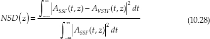
where and are the envelopes of the optical signals obtained by the SSFM and VSTF methods.
![]()
10.4 Transmission of Multiplexed Wavelength Channels
10.4.1 Dual Channel
The interchannel cross-talk induced by XPM, which is affected by channel spacing and the bit pattern of signal pulses, also plays an important part in the design of the DWDM systems. In order to demonstrate the applicability of the VSTF/S-VSTF model for the analysis of DWDM systems, a simplified dual-channel optical transmission system is implemented for simulation. Both the SSF method and the VSTF model are used for the simulation and their results compared.
In Section 10.3.1, the design setup of the dual-channel transmission system of 400 km transmission distance is discussed in detail. In Section 10.4.1, two sets of simulations are conducted to test the effect on cross-talk interference with different bit patterns. In Section 10.3.1, the effect of channel spacing is analyzed with the cross-phase modulation effects.
10.4.1.1 Transmission Systems
The design of the 400 km dual-channel transmission system is similar to the 400 km single-channel system implemented in this Section 10.4, with some modification. The dispersion compensation fiber (DCF) and nonzero dispersion shifted fiber (NZDSF) are interleaved to provide the needed dispersion management. Further, dispersion compensation is done at the end of the link with respect to each channel. The entire link consists of 5 sections of NZDSF, 5 sections of DCF, and 10 erbium-doped fiber amplifiers (EDFAs). Two channels of data-stream are multiplexed before transmitting and are demultiplexed at the end of the link. The schematic diagram of the optically amplified fiber transmission system setup is shown in Figure 10.3. The dispersion and attenuation spectrum of the NZDSF and DCF used in the link are listed in Table 10.1. The interleaving of NZDSF and DCF along the transmission link creates a zigzag pattern for the dispersion parameter (GVD). The variation of the dispersion and attenuation along the link can be easily estimated.
As expected the total dispersion experienced by Channel 1 and Channel 2 are quite different at the end of the transmission link. Therefore, it is necessary to have further dispersion compensation adjustment at the end of the link with respect to the amount of dispersion experienced by the channel. On the other hand, the attenuations for the two channels are almost identical. In the next section, the mathematical models developed in Section 10.2 are used for simulations. The XPM effect, a major factor contributing to the interchannel cross-talk, is investigated by simulation.
TABLE 10.1
Fiber Parameters for Nonzero Dispersion Shifted Fiber (NZDSF) and Dispersion Compensating Fiber (DCF)

10.4.1.2 Cross-Phase Modulation Effect and Bit Pattern Dependence
The XPM effect is the major contributor to the interchannel interference. Both the SPM and XPM are closely related to the intensity of the pulses transmitted. The bit pattern and channel spacing (in frequency) also play an important role in the XPM effect. In this section, the dual-channel transmission system proposed in Section 10.3.1 is used to simulate the pulse propagation of a dual-channel system. Different bit patterns are assigned to Channel 1 and Channel 2 in the first simulation, and then the bit pattern is changed for Channel 2 in the second simulation to facilitate comparison between the XPM caused by different bit patterns.
Case 1—Overlapped Pulse Sequence
In this case study, the following bit patterns are assigned for Channel 1 and Channel 2, respectively: (a1 and b1) Bit Pattern for Channel 1: [1 0 1 1]; and (a2 and b2) Bit Pattern for Channel 2: [1 1 0 0 ]. The evolution of the pulse sequences of Channel 1 and Channel 2 is shown in Figures 10.4a1 and 10.4b1 and Figures 10.4a2 and 10.4b2, respectively.
The discrepancy between the results obtained from the SSF method and the VSTF method is calculated using the NSD criterion given in (10.28). The NSD plots for both Channel 1 and Channel 2 are shown in Figure 10.5.
It is shown in Figure 10.5 that the VSTF method is adequate in representing the dual-channel optical transmission system. To examine the distortion caused by the XPM effect, the signal spectra of both Channel 1 and Channel 2 are plotted. The pulse spectra before and after transmission are plotted in Figures 10.6a1 and 10.6a2 and Figures 10.6b1 and 10.6b2, respectively.
Comparing the evolution of the pulse spectra of Figure 10.8, the distortion in Channel 2 is quite visible near the center of the carrier frequency. This is later to be compared to the spectrum obtained with a different bit pattern in Case 2.
Case 2—Nonoverlapped Pulse Sequence
In this simulation, the following bit patterns are assigned for Channel 1 and Channel 2, respectively: (a) Bit Pattern for Channel 1: [1 0 1 1]; and (b) Bit Pattern for Channel 2: [0 1 0 0]. There is no overlapping of the one-bit, and this should effectively reduce the XPM when both channels are in synchronization with each other. Due to the walk-off effect, the original frames of the two channels shift out of each other after the walk-off distance while other frames shift in along the transmission link.
The discrepancy between the results obtained from the SSF method and the VSTF model is calculated using the NSD criterion given in Equation (10.28). The NSD plots for both Channel 1 and Channel 2 are shown in Figures 10.7a and 10.7b. The NSD seems improved slightly as compared to those obtained in Case 1. This is due to the lower XPM effect. To compare the XPM distortion, the pulse spectrums before transmission and at the end of the link for Channel 1 and Channel 2, similar to Figure 10.6, are also obtained and analyzed for distortion. We can observe that the distortions experienced by both Channel 1 and Channel 2 are less. Thus, the bit pattern affects the contribution of XPM to the distortion of WDM transmission under the VSTF method.

FIGURE 10.4
Pulse evolution along transmission line of Channel 1 (a1,b1); Channel 2 (a2,b2) using (a1,a2) split-step Fourier method and (b1,b2) Volterra series transfer function model.
10.4.1.3 Cross-Phase Modulation and Channel Spacing
It was demonstrated that the bit patterns of the transmitting channels could affect the XPM effect. In this section, the relationship between the XPM effect and channel spacing is investigated. Instead of using 1550 nm and spaced by 100 GHz in frequency as the carrier frequencies, this spacing is halved in this section with the new carrier frequencies at 1550 nm and spaced by 50 GHz. The same NZDSF and DCF fibers of Table 10.1 are used for the simulation setup. A new variation of the dispersion and attenuation along the link is expected. It can be seen that the difference in dispersion increases due to the larger channel spacing. The obvious effect of the increased dispersion difference is the larger group velocity difference and hence shorter walk-off distance. It is noted that the dispersion factor and dispersion slope of the fibers employed in the transmission links are included in the NLSE.

FIGURE 10.5
Normalized squared deviation between split-step Fourier and Volterra series transfer function methods for both channels: (a) Channel 1, (b) Channel 2.
In this case study, the bit pattern used in Case 1 in Section 10.4.1.2 is used to facilitate the comparison with systems having different channel spacing. The following bit patterns are assigned for Channel 1 and Channel 2, respectively: (a) Bit Pattern for Channel 1: [1 0 1 1]; and (b) Bit Pattern for Channel 2: [1 1 0 0]. The pulse evolution for Channel 1 and Channel 2 are similarly obtained as given above. The discrepancy between the results obtained from the SSF and the VSTF methods is estimated using the NSD criterion. The NSD plots for both Channel 1 and Channel 2 are shown in Figure 10.8. The NSD obtained is similar in terms of magnitude as those obtained in Case 1. To compare the XPM distortion between the two simulations, the pulse spectrums before transmission and at the end of the link are, similar to Figure 10.6, also obtained and analyzed for distortion by both methods. The distortion experienced by Channel 2 is much less. Thus, it can be concluded that as the channel spacing increases, the contribution of XPM to the distortion of WDM transmission systems is less severe.

FIGURE 10.6
Normalized squared deviation power spectrum at the input launched end: (a1) Channel 1 and (a2) Channel 2, and at the output of pulse sequence under split-step Fourier and Volterra series transfer function methods for (b1) Channel 1 and (b2) Channel 2.
10.4.2 Triple Channel
The dual-channel optical transmission systems are simulated to investigate the effect of XPM and its relation with the bit pattern and channel spacing. In this section, the number of channels is three so that the effect of the overlapping of the bit pattern of either equal or uneven channel spacing between the channels can be examined. In this section the carrier frequencies of the three optical channels are selected to be equally spaced and nonequally spaced. The selected central wavelengths of the three channels are 1550 nm, 1555 nm, and 1560 nm. Each channel is 5 nm apart from the next channel. Closer spacing can be employed without minimum changes in the observed results. Then the carrier frequencies of the lowest and highest carriers are changed to 1549 nm and 1559 nm, thus channel spacing between Channel 1 and Channel 2, and 4 nm channel spacing between Channel 2 and Channel 3 is about 6 nm. The spacing is important for the case where the orthogonal frequency division multiplexed modulation schemes [21] are used in which the interactions between the subcarriers of different wavelength channels occur and can seriously affect the transmission quality.

FIGURE 10.7
Normalized squared deviation between split-step Fourier and Volterra series transfer function methods for Channels 1 and 2: (a) and (b), respectively.

FIGURE 10.8
Normalized squared deviation between split-step Fourier and Volterra series transfer function methods for both channels: (a) Channel 1, (b) Channel 2.
10.4.2.1 Equal Channel Spacing
The transmission setup for this simulation is similar to the systems used in Section 10.3.2. The schematic diagram is shown in Figure 10.9. Optical amplifiers, such as EDFAs are incorporated either at 40 km or 80 km span length. Raman optical amplification can also be included by the Raman scattering terms in the NLSE. The carriers of the three channels are located at frequencies 1550 nm (central frequency), and channel spaced by 50 GHz on the left and right sides of this wavelength. A noise figure of 3 dB is used for all optical amplification blocks. The bit patterns used for Channel 1, Channel 2, and Channel 3 are as follows: (a) Bit Pattern for Channel 1: [1 0 1 1]; (b) Bit Pattern for Channel 2: [1 1 0 0]; and (c) Bit Pattern for Channel 3: [0 1 0 1]. The propagation evolution of the bit patterns and NSD are plotted using similar methods given in Section 10.4.1.2. It is noted also that a total number of multiplexed channels is 40, which are located in the C-band catered at 1550 nm and spaced by 50 GHz between adjacent channels.
The evolution of the pulse sequences of the channels over 400 km transmission link of the three wavelength channels can be obtained via the S-VSTF model and the SSF model. The discrepancy between the results obtained from the SSF method and the VSTF model is calculated using the NSD criterion given by (10.28). The NSD plots for the three channels are shown in Figure 10.10.
In order to quantify the nonlinear distortion experienced by each channel, the following normalized distortion criterion is proposed:

where ch denotes the channel of interest; A( f, z) is the spectrum of the signal; f is the frequency variable; and z is the position.
Because the spectra are of a discrete form due to the periodic nature of the pulses, the summation is used in (10.29). The spectra at the beginning and the end of the fiber are normalized with respect to the total power, because only the shapes of the spectra are of interest for the nonlinear distortion analysis. Referring to Figure 10.11, we can observe that Channel 1 experiences less nonlinear distortion as compared to Channel 2 and Channel 3. This is due to the fact that the average power for Channel 1 is 50% higher as compared to the other two channels due to the assigned bit pattern. This shows that the XPM effects caused by other channels are more significant to the SPM effects caused by the channel itself.

FIGURE 10.9
The 400 km multichannel optic transmission system.

FIGURE 10.10
Normalized squared deviation plots of the three channels for the 400 km optic transmission system: (a) Channel 1, (b) Channel 2, and (c) Channel 3.
10.4.2.2 Unequal Channel Spacing
In Section 10.4.2.1, the optical transmission systems with three channels separated with equal channel spacing are simulated. In this section, unequal channel spacing is used to investigate the relation between XPM effects and channel spacing. The carriers of the three channels are located at wavelength 1555 nm (center channel) and spaced by 50 GHz on the left and 75 GHz the right frequency of the central wavelength. The GVD and attenuation of each channel can be evaluated from Table 10.1. The same bit pattern as used in Section 10.4.1.2 is employed in this simulation. The pulse evolution and NSD plots are depicted in Figure 10.12. The transmission was conducted over a 400 km link for three-multiplexed channels. Both VSTF and SSMF methods are used and compared. The evolution of the bit pattern over the propagation distance for the three channels under the VSTF model and SSFM can be obtained as illustrated in Figure 10.4. The discrepancy between the results obtained from the SSF method and the VSTF model is calculated using the NSD criterion given in (10.28). The NSD plots for the three channels are shown in Figure 10.12. To compare the nonlinear distortion caused by the XPM effects, the nonlinear distortion computed using (10.28) and (10.29) is illustrated in Figure 10.13 for the three channels. Comparing the nonlinear distortion plots of Figure 10.12 and Figure 10.13, it can be observed that the nonlinear distortion is reduced by only 50% under unequal channel spacing between the three channels.
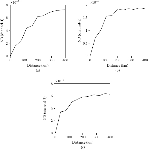
FIGURE 10.11
Nonlinear distortion of the three-channel transmission system: (a) Channel 1, (b) Channel 2, and (c) Channel 3.

FIGURE 10.12
Normalized squared deviation evolution over the 400 km optic transmission system for three channels: (a) Channel 1, (b) Channel 2, and (c) Channel 3.
10.4.3 Remarks
In this chapter, the segmented VSTF model is developed for evaluating the transmission performance of wavelength multiplexed systems. The method is also compared with the most popular method of the SSFM in representing the propagation of the optical pulse sequence over single-mode dispersive fibers. The mathematical model derived in Section 10.3 can be applied to DWDM systems with any number of channels. For simplicity, a dual-channel WDM system is simulated to demonstrate that the VSTF model can be adequate in design and analysis of a WDM transmission system. It has also been shown that both the bit pattern and the spacing between wavelength channels can affect the XPM effect, the leading contributor to the interchannel cross-talk. In Section 10.4.2, two different channel spacing schemes are used for the simulation. It has been shown that by tuning the carrier frequencies by a small amount to detune the equal channel spacing, the XPM effects can be reduced substantially. This nonlinear distortion is also evaluated with the restrictions defined as the difference between the VSTF and SSFM techniques.

FIGURE 10.13
Nonlinear distortion of the three-channel transmission system: (a) Channel 1, (b) Channel 2, and (c) Channel 3.
The segmentation of the fiber link is employed to ensure the convergence of the model as VSTF enabling the propagation of the optical pulse sequence over a very long length of fiber with minimum computing resources and time. However, the convergence of the VSTF influences the accuracy of the model. A dispersion criterion is given and coupled with the propagation of the pulses.
![]()
10.5 Inverse of Volterra Expansion and Nonlinearity Compensation in Electronic Domain
In this section, we describe compensation and equalization of nonlinear effects of optical signals transmitted over linear chromatic dispersion (CD) and nonlinear single-mode optical fiber. The mathematical representation of the equalization scheme is based on the inverse of the nonlinear transfer function represented by the Volterra series. The implementation of such a nonlinear equalization scheme is in the electronic domain. That is at the stage where the optical signals have been received and converted into the electrical domain as the voltage output of the electronic preamplifier, then digitized by an analog-to-digital converter (ADC) and processed in a digital signal processor.
The electronic nonlinearity compensation scheme based on the inverse of the Volterra expansion [30] is implemented in the electronic domain in a digital signal processor (DSP). It is first reported in Ip and Kahn [33] that 1.2 dB in quadrature (Q) improvement can be achieved with 256 Gb/s polarization division multiplexing (PDM)-16 quadrature amplitude modulation (QAM), and simultaneously reduce the compensation complexity by the reduction of the processing. To meet the ever-increasing demands of the data traffic, improvement in spectral efficiency is desired. Data signals modulate lightwaves via optical modulators using advanced modulation formats and multiplexing using subcarriers or polarization. Multilevel modulation formats such as 16QAM or 64QAM with higher spectrum efficiency are considered for realization of the future target rate of 400 Gb/s or 1Tb/s per channel. However, the multilevel modulation formats require that the received signal has a higher level of optical signal-to-noise ratio (OSNR) that significantly reduces the possible transmission distance. To achieve a higher received OSNR, suppression of the nonlinear penalty is inevitable to keep sufficient optical power from being launched into the transmission fiber. There are several approaches to suppress the nonlinearity such as dispersion management, employing new fibers with larger core diameter, and electronic nonlinear compensation in the digital domain. A typical structure of a digital coherent receiver for quadrature phase shift keying (QPSK) and polarization demultiplexing of optical channels is shown in Figure 10.14. First the optical channels are fed into a 90° hybrid coupler to mix with a local oscillator. Their polarizations are split so that they can be aligned for maximum efficiency. The opto-electronic device, a balanced pair of photodiodes, converts the optical into electronic currents and then is amplified by an electronic wideband preamplifier. At this stage the signals are in an electronic analog domain. The signals are then conditioned in their analog form (e.g., by an automatic gain control) and converted into digital quantized levels and processed by the digital signal processing unit.

FIGURE 10.14
Typical structure of a digital coherent receiver incorporating analog-to-digital converters (ADCs) and digital processing units. One ADC is assigned per detected channel of the in-phase and quadrature quantities.
Digital signal processing (DSP) techniques make possible the compensation of large amounts of accumulated chromatic dispersion at the receiver. As a result, we can achieve the benefit of suppressing interchannel nonlinearities in the WDM system by removing inline optical dispersion compensation, and hence reducing inline optical amplifiers and thus increasing or extending the transmission distance. Under this scenario, intrachannel nonlinearity becomes the dominant impairment [22]. Fortunately due to its deterministic nature, intrachannel nonlinearity can be compensated. Several approaches have been proposed to compensate the intrachannel nonlinearity, such as the digital back-propagation algorithm [23], the adaptive nonlinear equalization [24], and the maximum likelihood sequence estimation (MLSE) [25,26]. All of the proposed methods suffer from the difficulty that the implementation complexity is too high, especially their demands on ultrafast memory storage. In this chapter, we propose a new electronic nonlinearity compensation scheme based on the inverse of the Volterra expansion. We show that 1.2 dB in Q improvement can be achieved with 256 Gb/s PDM-16QAM transmission over a fiber link of 1000 km without inline dispersion compensation at 3 dBm launch power. We also simplify the implementation complexity by reducing the nonlinear processing rate. Negligible performance degradation with the same baud rate of the modulated data sequence for the nonlinearity compensation can also be achieved.
10.5.1 Inverse of Volterra Transfer Function
The Manakov-polarization mode dispersion (PMD) equations that describe the evolution of optical electromagnetic field envelope in an optical fiber operating in the nonlinear SPM (self-phase modulation) region can be expressed as [27]
![]()
![]()
where Ax and Ay are the electric field envelopes of the optical signals measured relative to the axes of the linear polarized mode of the fiber, β2 is the second-order dispersion parameter related to the group velocity dispersion (GVD) of the single-mode optical fiber, and α is the fiber attenuation coefficient. Both linear polarization-mode dispersion (PMD) and nonlinear polarization dispersion are not included for simplicity. The first- and third-order Volterra series transfer function for the solution of (10.30) and (10.31) can be written as [28]
![]()
![]()
where accounts for the impact of the waveform distortion due to the linear dispersion effects within a span. The complex term indicates the evolution of the phase of the carrier under the pulse envelope. The third-order kernel as a function of the nonlinear effects contains the main frequency component and the cross-coupling between different frequency components. Higher transfer functions H5 can be used as well, but consuming a large chunk of memory may not be possible for ultra-high-speed ADC and DSP chips. Furthermore, the accuracy of the contribution of this order function would not be sufficiently high to warrant its inclusion. When the linear dispersion is extracted, the third-order transfer function can be further simplified as
![]()
For optically amplified N spans fiber link without using the dispersion compensating module (DCM), the whole fiber transfer functions are given by [29]
![]()

where accounts for the waveform distortion at the input of each span. The third-order inverse kernel of this nonlinear system [30] can be obtained as
![]()

Taking the waveform distortion at the input of each span into consideration, and ignoring the waveform distortion within a span, (10.38) can be approximated by

10.5.2 Electronic Compensation Structure
Equations (10.37) and (10.39) can be realized by the scheme shown in Figure 10.15. This structure or algorithm can be implemented in the digital domain in the DSP after the electronic preamplifier and the ADC as described in Figure 10.14. Here is a constant, and compensates the residue dispersion of each span. Figure 10.15a shows the general structure to realize (10.37) and (10.39). The compensation can be separated into a linear compensation part and a nonlinear compensation part. The linear compensation part is simply CD compensation. The nonlinear compensation part can be divided into N stages, where N is the span number. The detailed realization of each nonlinear inverse compensating stage is shown in Figure 10.15b, which is a realization of
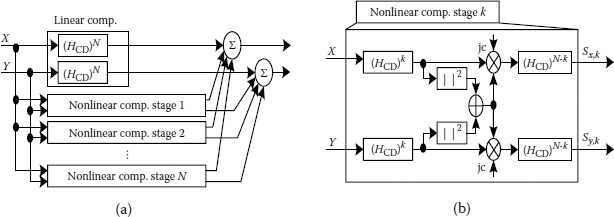
FIGURE 10.15
Electronic nonlinear compensation based on third-order inverse of Volterra expansion to be implemented in electronic digital signal processing: (a) block diagram of the proposed compensation scheme; (b) detailed realization of nonlinear compensation stage k. (Extracted from Ref [33]).
![]()


and are derived by first passing the received signal of X and Y through, and then implementing the nonlinear compensation of and [31]. Finally the residual dispersion can be compensated for by passing through the linear inverse function.
For linear compensation, the processing rate equal to doubling of the baud rate is common, but further reduction of the sampling rate can also be possible [31]. For the nonlinear compensation, it is possible by simulation that a single baud rate result is comparable to that of the doubling baud rate, hence reduction of the implementation complexity. It is very critical as the DSP at ultrahigh sampling rate is very limited in the number of numerical operations.

FIGURE 10.16
Simulation system setup and electronic nonlinearity compensation scheme at the digital coherent receiver with a nonlinear dispersion scheme in electronic domain employing the inverse Volterra series algorithm. (Extracted from Ref [33]).
The simulation platform is shown in Figure 10.16 [33]. The parameters of the transmission are also shown in the insert of Figure 10.16. The transmission scheme 256 Gb/s NRZ PDM-16QAM with periodically inserted pilots is generated at the transmitter and then transmitted through 13 spans of fiber link. Each span consists of a standard single-mode fiber (SSMF) with a CD coefficient of 16.8 ps/(nm.km), a Kerr nonlinearity coefficient of 0.0014 m–1W–1, a loss coefficient of 0.2 dB/km, and an EDFA with a noise figure of 5.5 dB. The span length is 80 km, and we assume 6 dB connector losses at the fiber span output, so the gain of each EDFA is 22 dB. There is also a preamplifier and a postamplifier at the transmitter and receiver to ensure a specified launch power and receiving power to satisfy the operational condition of the fiber nonlinear effects and the sensitivity of the coherent receiver. Random polarization rotation is also considered along the transmission line, but no polarization mode dispersion (PMD) is assumed. In order to have sufficient statistics, the same symbol sequence is transmitted 16 times with a different amplification stimulated emission (ASE) noise realization in the link and a total of 262,144 symbols are used for the estimation of the bit-error rate (BER). The transmitted signal is received with a polarization diversity coherent detector, then sampled at the rate of twice the baud rate and then processed in the digital electronic domain including the nonlinear inverse Volterra algorithm given herewith. The sampled signal first goes through the nonlinear compensator shown in Figure 10.16, where both CD and intrachannel nonlinearity are compensated. The quadruple butterfly-structured finite difference recursive filters and used for polarization demultiplexing and residual distortion compensation.Feed-forward carrier phase recovery is carried out before making a decision. With the help of periodically sent pilots, Gray mapping without differential coding can be used to minimize the complexity of the coder. The proposed nonlinear compensation scheme is shown in Figure 10.16. Both linear compensation and nonlinear compensation sections share the same first Fourier transform (FFT) and inverse (I) FFT to reduce the computing complexity. For the linear compensation, the processing rate is twice the baud rate. For the nonlinear compensation part, a reduced processing rate is possible to reduce the demand on the processing power of the DSP at extremely high speed.

FIGURE 10.17
Performance of the proposed nonlinearity compensator. Quality factor Q versus input launched power with and without nonlinearity compensator. (From L. Liu, L. Li, Y. Huang, and Q. Xiong, Electronic Nonlinearity Compensation of 256 Gb/s PDM-16QAM Based on Inverse of Volterra Expansion, submitted to IEEE Journal of Lightwave Technology. With permission.)
Figure 10.17 shows the performance of the proposed electronic nonlinear compensator. Figure 10.17 shows that the proposed nonlinearity compensator improves Q by 1.2 dB at 3 dBm launch power. This improvement is significant in terms of sensitivity of the receiver. It was found that [31] there is only negligible performance degradation with a nonlinear processing rate of the baud rate.
10.5.3 Remarks
In this section, an electronic digital processor is proposed with the processing algorithm based on the analytical version of the inverse Volterra series for compensation of the nonlinear effects in single-mode optical fibers in transmission systems. That is the optical modulated signals under polarization multiplexed 16-QAM scheme are transmitted over noncompensating fiber links and received by the optical receiver and sampled by a real-time oscilloscope and stored in memory for off-line processing.
The inverse of the Volterra transfer function of the fiber is derived from the nonlinear transfer function of the Volterra series of single-mode optical transmission lines. We showed that 1.2 dB Q improvement can be achieved with 256 Gb/s PDM-16QAM transmission over a fiber link of 1000 km without inline dispersion compensation and at 3 dBm launch power. The implementation complexity can be simplified with the reduction of the nonlinear processing rate. Negligible performance degradation with the sampling rate equals that of the baud rate for the nonlinearity compensation is also observed. When the high sampling rate ADC and compatible DSP integrated circuit (IC) are available, this algorithm would offer significant advantages in the real-time compensation of nonlinear propagation effects in the fiber transmission line. This electronic processing technique currently emerges as an advanced technology for enhancing the receiver sensitivity in association with a coherent detection method. The inverse Volterra transfer function is a nonlinear processing technique. The convergence of the inverse function must be further investigated to ensure that a solution is obtained within a finite time window.
![]()
References
1. J. E. Simsarian, J. Gripp, A. H. Gnauck, G. Raybon, and P. J. Winzer, Fast-Tuning 224-Gb/s Intradyne Receiver for Optical Packet Networks, OFC 2010, Postdeadline paper PDPB5, San Diego, Optical Fiber Conference 2010, March 2010.
2. T. D. Vo, Hao Hu, M. Galili, E. Palushani, J. Xu, L. K. Oxenløwe, S. J. Madden, D. Y. Choi, D. A. P. Bulla, M. D. Pelusi, J. Schröder1, B. Luther-Davies, and B. J. Eggleton, Photonic Chip Based 1.28 Tbaud Transmitter Optimization and Receiver OTDM Demultiplexing, OFC2010 Postdeadline paper PDPC5, Optical Fiber Conference 2010, San Diego, 2010.
3. G. Agrawal, Nonlinear Fiber Optics, 3rd ed., Academic Press, New York, 2002.
4. L. N. Binh, Digital Optical Communications, CRC Press, Boca Raton, FL, 2009.
5. M. Suzuki, T. Tsuritani, and N. Edagawa, Multi-Terabit Long Haul DWDM Transmission with VSB-RZ Format, IEEE LEOS Newsletter, October 2001, pp. 26–28.
6. N. Takachio and H. Suzuki, Application of Raman-Distributed Amplification to WDM Transmission Systems Using 1.55-µm Dispersion-Shifted Fiber, IEEE J. Lightwave Technol., 19(1), 60–69, January 2001.
7. V. Grigoryan and A. Richter, Efficient Approach for Modeling Collision-Induced Timing Jitter in WDM Return-to-Zero Dispersion-Managed Systems, IEEE J. Lightwave Technol., 18(8), 1148–1154, eq.2, August 2000.
8. K. P. Ho, Statistical Properties of Stimulated Raman Crosstalk in WDM Systems, IEEE J. Lightwave Technol., 18(7), 815–921, July 2000.
9. V. Grigoryan and A. Richter, Efficient Approach for Modeling Collision-Induced Timing Jitter in WDM Return-to-Zero Dispersion-Managed Systems, IEEE J. Lightwave Technol., 18(8), 1148–1154, August 2000.
10. K. Chang and L. Binh, A Simulation Platform for Single and Multi-Channel Transmission Systems in Frequency Domain Using Volterra Series Transfer Functions, Conference Proceedings, WARS02, Workshop on Applications of Radio Science, D3, Sydney NSW, Australia, 2002.
11. L. N. Binh, Linear and Nonlinear Transfer Functions of Single Mode Fiber for Optical Transmission Systems, J. Opt. Soc. Am. A, 26(7), 1564–1575, 2009.
12. K. V. Peddanarappagari and M. Brandt-Pearce, Volterra Series Transfer Function of Single-Mode Fibers, IEEE J. Lightwave Technol., 15(12), 2232–2241, 1997.
13. K. V. Peddanarappagari and M. Brandt-Pearce, Study of Fiber Nonlinearities in Communication Systems Using a Volterra Series Transfer Function Approach, Proc. 13th Annu. Conf. Inform. Sci-Syst., 752–757, 1997.
14. K. V. Peddanarappagari and M. Brandt-Pearce, Volterra Series Approach for Optimizing Fiber-Optic Communications System Designs, IEEE J. Lightwave Technol., 16(11), 2046–2055, 1998.
15. J. Tang, The Channel Capacity of a Multispan DWDM System Employing Dispersive Nonlinear Optical Fibers and an Ideal Coherent Optical Receiver, IEEE J. Lightwave Technol., 20(7), 1095–1101, 2002.
16. J. Tang, A Comparison Study of the Shannon Channel Capacity of Various Nonlinear Optical Fibers, IEEE J. Lightwave Technol., 24(5), 2070–2075, 2006.
17. J. Tang, The Shannon Channel Capacity of Dispersion-Free Nonlinear Optical Fiber Transmission, IEEE J. Lightwave Technol., 19(8), 1104–1109, 2001.
18. B. Xu and M. Brandt-Pearce, Comparison of FWM- and XPM-Induced Crosstalk Using the Volterra Series Transfer Function Method, IEEE J. Lightwave Technol., 21(1), 40–54, 2003.
19. L. N. Binh, On the Linear and Nonlinear Transfer Functions of Single Mode Fiber for Optical Transmission Systems, J. Opt. Soc. Am. A, 26(7), 1564–1575, 2009.
20. D. Atherton, Nonlinear Control Engineering, Van Nostrand Reinhold, New York, 1982.
21. W. Shieh and I. Djordjevic, OFDM for Optical Communications, Academic Press, New York, 2010.
22. E. Yamazaki et al., Mitigation of Nonlinearities in Optical Transmission Systems, OFC2011, OThF1, Optical Fiber Conference OFC 2001, Los Angeles, CA, March 6, 2001.
23. E. Ip and J. M. Kahn, Compensation of Dispersion and Nonlinear Impairments Using Digital Backpropagation, J. Lightwave Technol., 26(20), 3416–3425, October 2008.
24. Y. Gao et al., Experimental Demonstration of Nonlinear Electrical Equalizer to Mitigate Intra-channel Nonlinearities in Coherent QPSK Systems, ECOC2009, Vienna, Austria, Paper 9.4.7.
25. N. Stojanovic et al., MLSE-Based Nonlinearity Mitigation for WDM 112 Gbit/s PDM-QPSK Transmission with Digital Coherent Receiver, OFC2011, paper OWW6, Optical Fiber Conference OFC 2011, Los Angeles, CA, March 6, 2001.
26. L. N. Binh, T. L. Huynh, K. K. Pang, and Thiru Sivahumara, MLSE Equalizers for Frequency Discrimination Receiver of MSK Optical Transmission Systems, IEEE J. Lightwave Technol., 26(12), 1586–1595, June 15, 2008.
27. P. K. A. Wai et al., Analysis of Nonlinear Polarization-Mode Dispersion in Optical Fibers with Randomly Varying Birefringence, OFC’97, paper ThF4, 1997, Optical Fiber Conference OFC 97, Dallas, TX, USA.
28. K. V. Peddanarappagari and M. Brandt-Pearce, Volterra Series Transfer Function of Single-Mode Fibers, J. Lightwave Technol., 15(12), 2232–2241, December 1997.
29. J. K. Fischer et al., Equivalent Single-Span Model for Dispersion-Managed Fiber-Optic Transmission Systems, J. Lightwave Technol., 27(16), 3425–3432, August 2009.
30. M. Schetzen, Theory of pth-Order Inverse of Nonlinear Systems, IEEE Trans. on Circuits and Syst., 23(5), 285–291, May 1976.
31. E. Ip and J. M. Kahn, Digital Equalization of Chromatic Dispersion and Polarization Mode Dispersion, J. Lightwave Technol., 25(8), 2033–2043, August 2007.
32. T. Pfau et al., Hardware-Efficient Coherent Digital Receiver Concept with Feedforward Carrier Recovery for M-QAM Constellations, J. Lightwave Technol., 27(8), 989–999, April 2009.
33. L. Liu, L. Li, Y. Huang, and Q. Xiong, Electronic Nonlinearity Compensation of 256 Gb/s PDM-16QAM Based on Inverse of Volterra Expansion, submitted to IEEE Journal of Lightwave Technology.