Chapter 4

Regression I

4.1 Introduction

In this chapter, a nonparametric, rank-based (R) approach to regression modeling is presented. Our primary goal is the estimation of parameters in a linear regression model and associated inferences. As with the previous chapters, we generally discuss Wilcoxon analyses, while general scores are discussed in Section 4.4. These analyses generalize the rank-based approach for the two-sample location problem discussed in the previous chapter. Focus is on the use of the R package Rfit (Kloke and McKean 2012). We illustrate the estimation, diagnostics, and inference including confidence intervals and test for general linear hypotheses. We assume that the reader is familiar with the general concepts of regression analysis.

Rank-based (R) estimates for linear regression models were first considered by Jurečková (1971) and Jaeckel (1972). The geometry of the rank-based approach is similar to that of least squares as shown by McKean and Schrader (1980). In this chapter, the Rfit implementation for simple and multiple linear regression is discussed. The first two sections of this chapter present illustrative examples. We present a short introduction to the more technical aspects of rank-based regression in Section 4.4. The reader interested in a more detailed introduction is referred to Chapter 3 of Hettmansperger and McKean (2011).

We also discuss aligned rank tests in Section 4.5. Using the bootstrap for rank regression is conceptually the same as other types of regression and Section 4.6 demonstrates the Rfit implementation. Nonparametric Smoothers for regression models are considered in Section 4.7. In Section 4.8 correlation is presented, including the two commonly used nonparametric measures of association of Kendall and Spearman. In succeeding chapters we present rank-based ANOVA analyses and extend rank-based fitting to more general models.

4.2 Simple Linear Regression

In this section we present an example of how to utilize Rfit to obtain rank-based estimates of the parameters in a simple linear regression problem. Write the simple linear regression model as

$\begin{array}{ll}{Y}_i=\alpha +x_i\beta +e_i,\text{for}i=1,...n\hfill & (4.1)\hfill \end{array}$

where Yi is a continuous response variable for the ith subject or experimental unit, xi is the corresponding value of an explanatory variable, ei is the error term, α is an intercept parameter, and β is the slope parameter. Interest is on inference for the slope parameter β. The errors are assumed to be iid with pdf f(t). Closed form solutions exist for the least squares (LS) estimates of (4.1). However, in general, this is not true for rank-based (R) estimation.

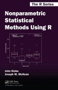
For the rest of this section we work with an example which highlights the use of Rfit. The dataset involved is engel which is in the package quantreg (Koenker 2013). The data are a sample of 235 Belgian working class households. The response variable is annual household income in Belgian francs and the explanatory variable is the annual food expenditure in Belgian francs.

A scatterplot of the data is presented in Figure 4.1 where the rank-based (R) and least squares (LS) fits are overlaid. Several outliers are present, which affect the LS fit. The data also appear to be heteroscedastic. The following code segment illustrates the creation of the graphic.

>  library(Rfit)

>  data(engel)

> plot(engel)

> abline(rfit(foodexp˜ income,data=engel))

> abline(lm(foodexp˜ income,data=engel),lty=2)

> legend(“topleft”,c(‘R’, ‘LS’) ,lty=c(1,2))

The command rfit obtains robust R estimates for the linear regression models, for example (4.1). To examine the coefficients of the fit, use the summary command. Critical values and p-values based on a Student t distribution with n − 2 degrees of freedom recommended for inference. For this example, Rfit used the t-distribution with 233 degrees of freedom to obtain the p-value.

>  fit<-rfit(foodexp˜ income,data=engel)

>  coef(summary(fit))

    Estimate Std. Error  t.value  p.value

(Intercept)  103.7667620 12.78877598 8.113893 2.812710e-14

income    0.5375705 0.01150719 46.716038 2.621879e-120

Readers with experience modeling in R will recognize that the syntax is similar to using lm to obtain a least squares analysis. The fitted regression equation is

$\widehat{\text{foodexp}}=103.767+0.538*\text{income}.$

A 95% confidence interval for the slope parameter (β) is calculated as 0.538 ± 1.97 * 0.012 = 0.538 ± 0.023 or (0.515, 0.56).

Examination of the residuals is an important part of the model building process. The raw residuals are available via the command residuals (fit), though we will focus on Studentized residuals. Recall that Studentized residuals are standardized so that they have an approximate (asymptotic) variance 1. In Figure 4.2, we present a residual plot as well as a normal probability plot of the Studentized residuals. The following code illustrates the creation of the graphic.

> rs<-rstudent(fit)

> yhat<-fitted.values(fit)

> par(mfrow=c(1,2))

> qqnorm(rs)

> plot(yhat,rs)

Outliers and heteroscedasticity are apparent in the residual and normal probability plots in Figure 4.2.

4.3 Multiple Linear Regression

Rank-based regression offers a complete inference for the multiple linear regression. In this section we illustrate how to use Rfit to obtain estimates, standard errors, inference and diagnostics based on an R fit of the model

$\begin{array}{ll}{Y}_i=\alpha +{\beta }_1{x}_{i1}+...{\beta }_p{x}_{ip}+e_i\text{for}i=1,...n\hfill & (4.2)\hfill \end{array}$

where β1,..., βp are regression coefficients, Yi is a continuous response variable, xi1,..., xip are a set of explanatory variables, ei is the error term, and α is an intercept parameter. Interest is on inference for the set of parameters β1,... βp. As in the simple linear model case, for inference, the errors are assumed to be iid with pdf f. Closed form solutions exist for the least squares (LS), however the R estimates must be solved iteratively.

4.3.1 Multiple Regression

In this subsection we discuss a dataset from Morrison (1983: p.64) (c.f. Hettmansperger and McKean 2011). The response variable is the level of free fatty acid (ffa) in a sample of prepubescent boys. The explanatory variables are age (in months), weight (in pounds), and skin fold thickness. In this subsection we illustrate the Wilcoxon analysis and in Exercise 4.9.3 the reader is asked to redo the analysis using bent scores. The model we wish to fit is

$\begin{array}{ll}\text{ffa}=\alpha +{\beta }_1\text{age}+{\beta }_2\text{weight}+{\beta }_3\text{skin}+\text{error}.\hfill & (4.3)\hfill \end{array}$

We use Rfit as follows to obtain the R fit of (4.3)

> fit<-rfit(ffa˜ age+weight+skin,data=ffa)

and a summary table may be obtained with the summary command.

> summary(fit)

Call:

rfit.default(formula = ffa ˜ age + weight + skin, data = ffa)

Coefficients:

   Estimate Std. Error t.value  p.value

(Intercept) 1.4900402 0.2692512 5.5340 2.686e-06 ***

age  -0.0011242 0.0026348 -0.4267 0.6720922

weight  -0.0153565 0.0038463 -3.9925 0.0002981 ***

skin  0.2749014 0.1342149 2.0482 0.0476841 *

–––

Signif. codes: 0 ‘***’ 0.001 ‘**’ 0.01 ‘*’ 0.05 ‘.’ 0.1 ‘ ’ 1

Multiple R-squared (Robust): 0.3757965

Reduction in Dispersion Test: 7.42518 p-value: 0.00052

Displayed are estimates, standard errors, and Wald (t-ratio) tests for each of the individual parameters. The variable age is nonsignificant, while weight and skin fold thickness are. In addition there is a robust R2 value which can be utilized in a manner similar to the usual R2 value of LS analysis; here R2 = 0.38. Finally a test of all the regression coefficients excluding the intercept parameter is provided in the form of a reduction in dispersion test. In this example, we would reject the null hypothesis and conclude that at least one of the nonintercept coefficients is a significant predictor of free fatty acid.

The reduction in dispersion test is analogous to the LS’s F-test based on the reduction in sums of squares. This test is based on the reduction (drop) in dispersion as we move from the reduced model (full model constrained by the null hypothesis) to the full model. As an example, for the free fatty acid data, suppose that we want to test the hypothesis:

$\begin{array}{ll}{H}_0:{\beta }_{\text{age}}={\beta }_{\text{weight}}=0\text{versus}{H}_A:{\beta }_{\text{age}}\ne 0\text{or}{\beta }_{\text{weight}}\ne 0.\hfill & (4.4)\hfill \end{array}$

Here, the reduced model contains only the regression coefficient of the predictor skin, while the full model contains all three predictors. The following code segment computes the reduction in dispersion test, returning the F test statistic (see expression (4.15)) and the corresponding p-value:

>  fitF<-rfit(ffa˜ age+weight+skin,data=ffa)

>  fitR<-rfit(ffa˜ skin,data=ffa)

>  drop.test(fitF,fitR)

Drop in Dispersion Test

F-Statistic p-value

 1.0768e+01  2.0624e-04

The command drop.test was designed with the functionality of the command anova in traditional analyses in mind. In this case, as the p-value is small, the null hypothesis would be rejected at all reasonable levels of α.

4.3.2 Polynomial Regression

In this section we present an example of a polynomial regression fit using Rfit. The data are from Exercise 5 of Chapter 10 of Higgins (2003). The scatterplot of the data in Figure 4.3 reveals a curvature relationship between MPG (mpg) and speed (sp). Higgins (2003) suggests a quadratic fit and that is how we proceed. That is, we fit the model

$\text{speed}=\alpha +{\beta }_1\text{mpg}+{\beta }_2{\text{mpg}}^2+\text{error}.$

To specify a squared term (or any function of the data to be interpreted arithmetically) use the I function:

> summary(fit<-rfit(sp˜ mpg+I(mpg^2),data=speed))

Call :

rfit.default(formula = sp mpg + I(mpg^2), data = speed)

Coefficients :

   Estimate  Std. Error t.value p.value

(Intercept) 160.7246773 6.4689781 24.8455 < 2.2e-16 ***

mpg  -2.1952729 0.3588436 -6.1176 3.427e-08 ***

I(mpg^2)  0.0191325 0.0047861 3.9975 0.000143 ***

–––

Signif. codes: 0 ‘***’ 0.001 ‘**’ 0.01 ‘*’ 0.05 ‘.’ 0.1 ‘ ’ 1

Multiple R-squared (Robust): 0.5419925

Reduction in Dispersion Test: 46.74312 p-value: 0

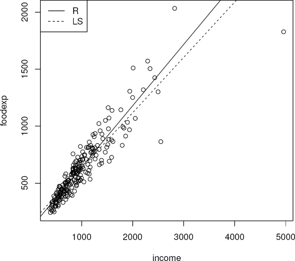
Note that the quadratic term is highly significant. The residual plot, Figure 4.4, suggests that there is the possibility of heteroscedasticity and/or outliers; however, there is no apparent lack of fit.

Remark 4.3.1 (Model Selection).

For rank-based regression, model selection can be performed using forward, backwards, or step-wise procedures in the same way as in ordinary least squares. Procedures for penalized rank-based regression have been developed by Johnson and Peng (2008). In future versions of Rfit we plan to include penalized model selection procedures.

4.4 Linear Models*

In this section we provide a brief overview of rank-based methods for linear models. Our presentation is by no means comprehensive and is included simply as a convenient reference. We refer the reader interested in a thorough treatment to Chapters 3,–5 of Hettmansperger and McKean (2011). This section uses a matrix formulation of the linear model; readers interested in application can skip this and the next section.

4.4.1 Estimation

In this section we discuss rank-based (R) estimation for linear regression models. As is the case with most of the modeling we discuss in this book, the geometry is similar to least squares. Throughout we are interested in estimation and inference on the slope parameters in the following linear model

$\begin{array}{ll}{Y}_i=\alpha +{\beta }_1{x}_{i1}+...+{\beta }_p{x}_{ip}+e_i\text{for}i=1,...,n.\hfill & (4.5)\hfill \end{array}$

For convenience we rewrite (4.5) as

$\begin{array}{ll}{Y}_i=\alpha +x_i^T\beta +e_i\text{for}i=1,...,n,\hfill & (4.6)\hfill \end{array}$

where Yi is a continuous response variable, xi is the vector of explanatory variables, α is the intercept parameter, β is the vector of regression coefficients, and ei is the error term. For formal inference, the errors are assumed to be iid with continuous pdf f(t) and finite Fisher information. Additionally, there are design assumptions that are the same as those for the least squares analysis.

Rewrite (4.6) in matrix notation as follows

$\begin{array}{ll}\mathit{Y}=\alpha \mathbf{1}+\mathit{X}\beta +e\hfill & (4.7)\hfill \end{array}$

where $\mathit{Y}={[Y_1,...,Y_n]}^T$is a n × 1 vector of response variable, $\mathit{X}={\left[x_1,...,x_n\right]}^T$ is an n × p design matrix, and $\mathit{e}={\left[e_1,...,e_n\right]}^T$ is an n × 1 vector of error terms. Recall that the least squares estimator is the minimizer of Euclidean distance between Y and ${\widehat{\mathit{Y}}}_{LS}=\mathit{X}{\widehat{\beta }}_{LS}$. To obtain the R estimator, we use a different measure of distance, Jaeckel’s (1972) dispersion function, which is given by:

$\begin{array}{ll}D\left(\beta \right)={||\mathit{Y}-\mathit{X}\beta ||}_{\phi },\hfill & (4.8)\hfill \end{array}$

where ${||\cdot ||}_{\phi }$ is a pseudo-norm defined as

$\begin{array}{ll}{||\mathit{u}||}_{\phi }={\displaystyle \sum _{i=1}^{n}a(R(u_i))u_i,}\hfill & (4.9)\hfill \end{array}$

the scores are generated as $a\left(i\right)=\phi \left(\frac{i}{n+1}\right)$, and φ is a nondecreasing score function defined on the interval (0,1). Any of the score functions discussed in the previous chapter for the two-sample location problem can be used in a linear model setting and, therefore, in any of the models used in the remainder of this book. An adaptive procedure for the regression problem is discussed in Section 7.6.

It follows that D(β), (4.8), is a convex function of β and provides a robust measure of distance between Y and Xβ. The R estimator of β is defined as

$\begin{array}{ll}{\widehat{\beta }}_{\phi }=\text{Argmin}{||\mathit{Y}-\mathit{X}\beta ||}_{\phi }.\hfill & (4.10)\hfill \end{array}$

Note that closed form solutions exist for least squares, however, this is not the case for rank estimation. The R estimates are obtained by minimizing a convex optimization problem. In Rfit, the R function optim is used to obtain the estimate of β.

It can be shown, see for example Hettmansperger and McKean (2011), that the solution to (4.10) is consistent with the asymptotically normal distribution given by

$\begin{array}{ll}{\widehat{\beta }}_{\phi }\dot{~}N\left(\beta ,{\tau }_{\phi }^2{\left({\mathit{X}}^T\mathit{X}\right)}^{-1}\right),\hfill & (4.11)\hfill \end{array}$

where τφ is the scale parameter which is defined in expression (3.19). Note that τφ depends on the pdf f(t) and the score function φ(u). In Rfit, the Koul, Sievers, and McKean (1987) consistent estimator of τφ is computed.

The intercept parameter, α, is estimated separately using a rank-based estimate of location based on the residuals $y_i-x_i^T{\widehat{\beta }}_{\phi }$. Generally the median is used, which is the default in Rfit, and which we denote by $\widehat{\alpha }$. It follows that $\widehat{\alpha }$ and ${\widehat{\beta }}_{\phi }$ are jointly asymptotically normal with the variance-covariance matrix

$\begin{array}{cc}{\mathit{V}}_{\widehat{\alpha },{\widehat{\beta }}_{\phi }}=\left[\begin{array}{cc}{\kappa }_n& -{\tau }_{\phi }^2{\overline{\mathit{x}}}^{\prime }{({\mathit{X}}^{\prime }\mathit{X})}^{-1}\\ -{\tau }_{\phi }^2{({\mathit{X}}^{\prime }\mathit{X})}^{-1}\overline{\mathit{x}}& {\tau }_{\phi }^2{({\mathit{X}}^{\prime }\mathit{X})}^{-1}\end{array}\right],& (4.12)\end{array}$

where ${\kappa }_n=n^{-1}{\tau }_S^2+{\tau }_{\phi }^2{\overline{x}}^{\prime }{\left({\mathit{X}}^{\prime }\mathit{X}\right)}^{-1}\overline{x}$. The vector $\overline{x}$ is the vector of column averages of X and τS is the scale parameter1 1/[2f(0)]. The consistent estimator of τS, discussed in Section 1.5 of Hettmansperger and McKean (2011), is implemented in Rfit.

4.4.2 Diagnostics

Regression diagnostics are an essential part of the statistical analysis of any data analysis problem. In this section we discuss Studentized residuals. Denote the residuals from the full model fit as

$\begin{array}{cc}{\widehat{e}}_i=Y_i-\widehat{\alpha }-x_i\widehat{\beta }.& (4.13)\end{array}$

Then the Studentized residuals are defined as

$\frac{{\widehat{e}}_i}{s\left({\widehat{e}}_i\right)}$

where $s\left({\widehat{e}}_i\right)$ is the estimated standard error of ${\widehat{e}}_i$ discussed in Chapter 3 of Hettmansperger and McKean (2011). In Rfit, the command rstudent is used to obtain Studentized residuals from an R fit of a linear model.

4.4.3 Inference

Based on the asymptotic distribution of ${\widehat{\beta }}_{\phi }$, (4.11), we present inference for the vector of parameters β. We discuss Wald type confidence intervals and tests of hypothesis. In addition to these procedures, R-analyses offer the drop in dispersion test which is an analog of the traditional LS test based on the reduction in sums of squares. An estimate of the scale parameter τφ is needed for inference and the Koul et al. (1987) estimator is implemented in Rfit.

From (4.11), Wald tests and confidence regions/intervals can easily be obtained. Let se$\left({\widehat{\beta }}_j\right)$ denote the standard error of ${\widehat{\beta }}_j$. That is se$\left({\widehat{\beta }}_j\right)={\widehat{\tau }}_{\phi }{\left({\mathit{X}}^T\mathit{X}\right)}_{jj}^{-1/2}$ where ${\left({\mathit{X}}^T\mathit{X}\right)}_{jj}^{-1}$ is the jth diagonal element of (XT X)−1.

An approximate (1 - α) * 100% confidence interval for βj is

${\widehat{\beta }}_j\pm t_{1-\alpha /2,n-p-1}\text{se}\left({\widehat{\beta }}_j\right).$

A Wald test of the hypothesis

$\begin{array}{cc}{H}_0:M\beta =\mathbf{0}\text{versus}{H}_A:M\beta \ne \mathbf{0}& (4.14)\end{array}$

is to reject H0 if

$\frac{{\left(M{\widehat{\beta }}_{\phi }\right)}^T{[M{({\mathit{X}}^T\mathit{X})}^{-1}{\mathit{M}}^T]}^{-1}(\mathit{M}\widehat{\beta })/q}{{\widehat{\tau }}_{\phi }^2}>F_{1-\alpha ,q,n-p-1}$

where q = dim(M).

Similar to the reduction in the sums of squares test of classical regression, rank-based regression offers a drop in dispersion test. Let ΩF denote the full model space; i.e., the range (column space) of the design matrix X for the full Model (4.7). Let D(FULL) denote the minimized value of the dispersion function when the full model (4.7) is fit. That is, $D\left(\text{FULL}\right)=D\left({\widehat{\beta }}_{\phi }\right)$. Geometrically, D(FULL) is the distance between the response vector y and the space ΩF. Let ΩR denote the reduced model subspace of ΩF; that is, ${\mathrm{\Omega }}_R=\left\{\upsilon \in {\mathrm{\Omega }}_F:\upsilon =\mathit{X}\beta \text{and}\mathit{M}\beta =0\right\}$. Let D(RED) denote the minimum value of the dispersion function when the reduced model is fit; i.e., D(RED) is the distance between the response vector y and the space ΩR. The reduction in dispersion is $RD=D\left(RED\right)-D\left(FULL\right)$. The drop in dispersion test is a standardization of the reduction in dispersion which is given by

$\begin{array}{cc}{F}_{\phi }=\frac{\text{RD}/q}{\widehat{\tau }/2}.& (4.15)\end{array}$

An approximate level α test is to reject H0 if

$\begin{array}{cc}{F}_{\phi }=\frac{\text{RD}/q}{\widehat{\tau }/2}>F_{1-\alpha ,q,n-p-1}.& (4.16)\end{array}$

The default ANOVA and ANCOVA Rfit analyses described in Chapter 5 use Type III general linear hypotheses (effect being tested is adjusted for all other effects). The Wald type test satisfies this by its formulation. This is true also of the drop in dispersion test defined above; i.e., the reduction in dispersion is between the reduced and full models. Of course, the reduced model design matrix must be computed. This is easily done, however, by using a QR-decomposition of the row space of the hypothesis matrix M; see page 210 of Hettmansperger and McKean (2011). For default tests, Rfit uses this development to compute a reduced model design matrix for a specified matrix M. In general, the Rfit function redmod(xmat,amat) computes a reduced model design matrix for the full model design matrix xfull and the hypothesis matrix amat. For traditional LS tests, the corresponding reduction in sums-of-squares is often refereed to as a Type III sums-of-squares.

4.4.4 Confidence Interval for a Mean Response

Consider the general linear model (4.7). Let x0 be a specified vector of the independent variables. Although we need not assume finite expectation of the random errors, we do in this section, which allows us to use familiar notation. In practice, a problem of interest is to estimate ${\eta }_0=E\left(Y|x_0\right)$ for a specified vector of predictors x0. We next consider solutions for this problem based on a rank-based fit of Model (4.7). Denote the rank-based estimates of α and β by $\widehat{\alpha }$ and $\widehat{\beta }$.

The estimator of η0 is of course

$\begin{array}{cc}{\widehat{\eta }}_0=\widehat{\alpha }+x_0^T\widehat{\beta }.& (4.17)\end{array}$

It follows that ${\widehat{\eta }}_0$ is asymptotically normal with mean η0 and variance, using expression (4.12),

$\begin{array}{cc}{\upsilon }_0=\text{Var}\left({\widehat{\eta }}_0\right)=[1x_0^T]{\widehat{\mathit{V}}}_{\widehat{\alpha },{\widehat{\beta }}_{\phi }}\left[\begin{array}{c}1\\ x_0\end{array}\right].& (4.18)\end{array}$

Hence, an approximate (1 − α) 100% confidence interval for η0 is

$\begin{array}{cc}{\widehat{\eta }}_0\pm t_{\alpha /2,n-p-1}\sqrt{{\widehat{\upsilon }}_0},& (4.19)\end{array}$

where ${\widehat{\upsilon }}_0$ is the estimate of v0, (τs and τφ are replaced respectively by ${\widehat{\tau }}_S$ and ${\widehat{\tau }}_{\phi }$).

Using Rfit this confidence interval is easily computed. Suppose x0 contain the explanatory variables for which we want to estimate the mean response. The following illustrates how to obtain the estimate and standard error, from which a confidence interval can be computed. Assume the full model fit has been obtained and is in fit (e.g. fit<-rfit(y˜ X)).

x10 <- c(1,x0)

st. err <- sqrt(t (x10)%*%vcov(f it)%*%x10)

eta0 <- t (x10)%*%f it$coef

We illustrate this code with the following example.

Example 4.4.1.

The following responses were collected consecutively over time. For convenience take the vector of time to be t <- 1:15.

Interest centered on the model for linear trend, $y=\alpha +\beta t+e$, and in estimating the expected value of the response for the next time period t = 16. Using Wilcoxon scores and the above code, Exercise 4.9.7 shows that predicted value at time 16 is 5.43 with the 95% confidence interval (3.38, 7.48). Note in practice this might be considered an extrapolation and consideration must be made as to whether the time trend will continue.

There is a related problem consisting of a predictive interval for Y0 a new (independent of Y) response variable which follows the linear model at x0. Note that Y0 has mean η0. Assume finite variance, σ2, of the random errors. Then $Y_0-\widehat{\eta }$ has mean 0 and (asymptotic) variance σ2 + v0, where v0 is given in expression (4.19). If in addition we assume that the random errors have a normal distribution, then we could assume (asymptotically) that the difference $Y_0-\widehat{\eta }$ is normally distributed. Based on these results a predictive interval is easily formed. There are two difficult problems here. One is the assumption of normality and the second is the robust estimation of σ2. Preliminary Monte Carlo results show that estimation of σ by MAD of the residuals leads to liberal predictive intervals. Also, we certainly would not recommend using the sample variance of robust residuals. Currently, we are investigating a bootstrap procedure.

4.5 Aligned Rank Tests*

An aligned rank test is a nonparametric method which allows for adjustment of covariates in tests of hypotheses. In the context of a randomized experiment to assess the effect of some intervention one might want to adjust for baseline covariates in the test for the intervention. In perhaps the simplest context of a two-sample problem, the test is based on the Wilcoxon rank sum from the residuals of a robust fit of a model on the covariates. Aligned rank tests were first developed by Hodges and Lehmann (1962) for use in randomized block designs. They were developed for the linear model by Adichie (1978); see also Puri and Sen (1985) and Chiang and Puri (1984). Kloke and Cook (2014) discuss aligned rank tests and consider an adaptive scheme in the context of a clinical trial.

For simplicity, suppose that we are testing a treatment effect and each subject is randomized to one of k treatments. For this section consider the model

$\begin{array}{cc}{Y}_i=\alpha +{\mathit{w}}_i^T\mathbf{\Delta }+x_i^T\beta +e_i& (4.20)\end{array}$

where wi is a (k–1) × 1 incidence vector denoting the treatment assignment for the ith subject, $\mathbf{\Delta }={\left[{\mathrm{\Delta }}_2,...,{\mathrm{\Delta }}_K\right]}^T$ is a vector of unknown treatment effects, xi is a p × 1 vector of (baseline) covariates, β is a vector of unknown regression coefficients, and ei denotes the error term. The goal of the experiment is to test

$\begin{array}{cc}{H}_0:\mathbf{\Delta }=\mathbf{0}.& (4.21)\end{array}$

In this section we focus on developing an aligned rank tests for Model (4.20). We write the model as

$\begin{array}{cc}\mathit{Y}=\alpha \mathbf{1}+\mathit{W}\mathbf{\Delta }+\mathit{X}\beta +e=\alpha \mathbf{1}+\mathit{Z}\mathit{b}+e.& (4.22)\end{array}$

Then the full model gradient is

$\mathit{S}\left(\mathit{b}\right)={\mathit{Z}}^T\mathit{a}(R(\mathit{Y}-\mathit{Z}\mathit{b})).$

First, fit the reduced model

$\mathit{Y}=\alpha 1+\mathit{X}\beta +e.$

Then plug the reduced model estimate ${\widehat{b}}_r={\left[0^T{\widehat{\beta }}_r^T\right]}^T$ into the full model:

$\mathit{S}\left({\widehat{\mathit{b}}}_{\tau }\right)\dot{=}\left[\begin{array}{c}{\mathit{W}}^{T}a(R(\mathit{Y}-\mathit{X}{\widehat{\beta }}_{\tau }))\\ 0\end{array}\right].$

Define ${\widehat{\mathit{S}}}_1={\mathit{W}}^{T}a\left(R\left(\mathit{Y}-\mathit{X}{\widehat{\beta }}_r\right)\right)$ as the first k – 1 elements of $\mathit{S}\left({\widehat{b}}_r\right)$. Then the aligned rank test for (4.21) is based on the test statistic

${\widehat{\mathit{S}}}_1^T{[{\mathit{W}}^T\mathit{W}-{\mathit{W}}^T{\mathit{H}}_{\mathit{X}}\mathit{W}]}^{-1}{\widehat{\mathit{S}}}_1={\widehat{\mathit{S}}}_1^T{[{\mathit{W}}^T{\mathit{H}}_{{\mathit{X}}^{\perp }}\mathit{W}]}^{-1}{\widehat{\mathit{S}}}_1$

where HX is the projection matrix onto the space spanned by the columns of X. For inference, this test statistic should compared to ${\chi }_{K-1}^2$ critical values.

In the package npsm, we have included the function aligned.test which performs the aligned rank test.

A simple simulated example illustrates the use of the code.

> k<-3  # number of treatments

> p<-2  # number of covariates

> n<-10 # number of subjects per treatment

> N<-n*k # total sample size

> y<-rnorm (N)

> x<-matrix(rnorm(N*p),ncol=p)

> g<-rep(1:k,each=n)

> aligned.test(x,y,g)

statistic = 1.083695 , p-value = 0.5816726

4.6 Bootstrap

In this section we illustrate the use of the bootstrap for rank-based (R) regression. Bootstrap approaches for M estimation are discussed in Fox and Weisberg (2011) and we take a similar approach. While it is not difficult to write bootstrap functions in R, we make use of the boot library. Our goal is not a comprehensive treatment of the bootstrap, but rather we present an example to illustrate its use.

In this section we utilize the baseball data, which is a sample of 59 professional baseball players. For this particular example we regress the weight of a baseball player on his height.

To use the boot function, we first define a function from which boot can calculate bootstrap estimates of the regression coefficients:

> boot.rfit<-function(data,indices) {

+ data<-data[indices,]

+ fit<-rfit(weight˜ height,data=data,tau=‘N’)

+ coefficients(fit)[2]

+}

Next use boot to obtain the bootstrap estimates, etc.

> bb.boot<-boot(data=baseball,statistic=boot.rfit,R=1000)

> bb.boot

ORDINARY NONPARAMETRIC BOOTSTRAP

Call:

boot(data = baseball, statistic = boot.rfit, R = 1000)

Bootstrap Statistics :

 original bias std. error

t1* 5.714278 -0.1575826  0.7761589

Our analysis is based on 1000 bootstrap replicates.

Figure 4.5 shows a histogram of the bootstrap estimates and a normal probability plot.

> plot(bb.boot)

Bootstrap confidence intervals are obtained using the boot.ci command. In this segment we obtain the bootstrap confidence interval for the slope parameter.

> boot.ci(bb.boot,type=‘perc’,index=1)

BOOTSTRAP CONFIDENCE INTERVAL CALCULATIONS

Based on 1000 bootstrap replicates

CALL :

boot.ci(boot.out = bb.boot, type = “perc”, index = 1)

Intervals :

Level Percentile

95%  (3.75, 7.00)

Calculations and Intervals on Original Scale

Exercise 4.9.4 asks the reader to compare the results with those obtained using large sample inference.

4.7 Nonparametric Regression

In this chapter we have been discussing linear models. Letting Yi and $x_i={\left[x_{i1},...,x_{ip}\right]}^T$ denote the ith response and its associated vector of explanatory variables, respectively, these models are written as

$\begin{array}{cc}{Y}_i=\alpha +{\beta }_1{x}_{i1}+{\beta }_2{x}_{i2}+\cdots +{\beta }_p{x}_{ip}+e_i,i=1,...,n.& (4.23)\end{array}$

Note that these models are linear in the regression parameters ${\beta }_{j}j=1,...,p$; hence, the name linear models. Next consider the model

$\begin{array}{cc}{Y}_i={\beta }_1\exp \{\alpha +{\beta }_2{x}_{i1}+{\beta }_3{x}_{i3}\}+e_i,i=1,...,n.& (4.24)\end{array}$

This model is not linear in the parameters and is an example of a nonlinear model. We explore such models in Section 7.7. The form of Model (4.24) is still known. What if, however, we do not know the functional form? For example, consider the model

$\begin{array}{cc}{Y}_i=g\left(x_i\right)+e_i,i=1,...,n,& (4.25)\end{array}$

where the function g is unknown. This model is often called a nonparamet-ric regression model. There can be more than one explanatory variable xi, but in this text we only consider one predictor. As with linear models, the goal is to fit the model. The fit usually shows local trends in the data, finding peaks and valleys which may have practical consequences. Further, based on the fit, residuals are formed to investigate the quality of fit. This is the main topic of this section. Before turning our attention to nonparametric regression models, we briefly consider polynomial models. We consider the case of unknown degree, so, although they are parametric models, they are not completely specified.

4.7.1 Polynomial Models

Suppose we are willing to assume that g(x) is a sufficiently smooth function. Then by Taylor’s Theorem, a polynomial may result in a good fit. Hence, consider polynomial models of the form

$\begin{array}{cc}{Y}_i=\alpha +{\beta }_1\left(x_i-\overline{x}\right)+{\beta }_2{\left(x_i-\overline{x}\right)}^2+\cdots +{\beta }_p{\left(x_i-\overline{x}\right)}^p+e_i,i=1,...,n,& (4.26)\end{array}$

Here x is centered as shown in the model. A disadvantage of this model is that generally the degree of the polynomial is not known. One way of dealing with this unknown degree is to use residual plots based upon iteratively fitting polynomials of different degrees to determine a best fit; see Exercise 4.9.10 for such an example.

To determine the degree of a polynomial model, Graybill (1976) suggested an algorithm based on testing for the degree. Select a large (super) degree P which provides a satisfactory fit of the model. Then set p = P, fit the model, and test βp = 0. If the hypothesis is rejected, stop and declare p to be the degree. If not, replace p with p − 1 and reiterate the test. Terpstra and McKean (2005) discuss the results of a small simulation study which confirmed the robustness of the Wilcoxon version of this algorithm. The npsm package contains the R function polydeg which performs this Wilcoxon version. We illustrate its use in the following example based on simulated data. In this section, we often use simulated data to check how well the procedures fit the model.

Example 4.7.1 (Simulated Polynomial Model).

In this example we simulated data from the the polynomial $g\left(x\right)=10-3x-3x^3+x^3$. One-hundred x values were generated from a N(0, 3)-distribution while the added random noise, ei, was generated from a t-distribution with 2 degrees of freedom and with a multiplicative scale factor of 15. The data are in the set poly. The next code segment shows the call to polydeg and the resulting output summary of each of its steps, consisting of the degree tested, the drop in dispersion test statistic, and the p-value of the test. Note that we set the super degree of the polynomial to 5.

> deg<-polydeg(x,y,5, .05)

> deg$coll

 Deg  Robust F  p-value

  5 2.331126  0.1301680

  4 0.474083  0.4927928

  3 229.710860 0.0000000

> summary(deg$fitf)

Call :

rfit.default(formula = y ˜ xmat)

Coefficients :

   Estimate Std. Error t.value  p.value

(Intercept)  9.501270  3.452188 2.7522 0.007077 **

xmatxc  -7.119670  1.247642 -5.7065 1.279e-07 ***

xmat  -1.580433  0.212938 -7.4220 4.651e-11 ***

xmat  1.078679  0.045958 23.4707 < 2.2e-16 ***

–––

Signif. codes: 0 ‘***’ 0.001 ‘**’ 0.01 ‘*’ 0.05 ‘.’ 0.1 ‘ ’ 1

Multiple R-squared (Robust): 0.7751821

Reduction in Dispersion Test: 110.3375 p-value: 0

Note that the routine determined the correct degree; i.e., a cubic. Based on the summary of the cubic fit, the 95% confidence interval for the leading coefficient β3 traps its true value of 1. To check the linear and quadratic coefficients, the centered polynomial must be expanded. Figure 4.6 displays the scatterplot of the data overlaid by the rank-based fit of the cubic polynomial and the associated Studentized residual plot. The fit appears to be good which is confirmed by the random scatter of the Studentized residual plot. This plot also identifies several large outliers in the data, as expected, because the random errors follow a t-distribution with 2 degrees of freedom.

4.7.2 Nonparametric Regression

There are situations where polynomial fits will not suffice; for example, a dataset with many peaks and valleys. In this section, we turn our attention to the nonparametric regression model (4.25) and consider several nonparametric procedures which fit this model. There are many references for nonparametric regression models. An informative introduction, using R, is Chapter 11 of Faraway (2006); for a more authoritative account see, for example, Wood (2006). Wahba (1990) offers a technical introduction to smoothing splines using reproducing kernel Hilbert spaces.

Nonparametric regression procedures fit local trends producing, hopefully, a smooth fit. Sometimes they are called smoothers. A simple example is provided by a running average of size 3. In this case the fit at xi is (Yi−1 + Yi + Yi+1)/3. Due to the non-robustness of this fit, often the mean is replaced by the median.

The moving average can be thought of as a weighted average using the discrete distribution with mass sizes of 1/3 for the weights. This has been generalized to using continuous pdfs for the weighting. The density function used is called a kernel and the resulting fit is called a kernel nonparametric regression estimator. One such kernel estimator, available in base R, is the Nadaraya–Watson estimator which is defined at x by

$\begin{array}{cc}{\widehat{f}}_h\left(x\right)=\frac{1}{nh}{\displaystyle \sum _{i=1}^n\frac{w_i}{{\displaystyle {\sum }_{j=1}^n{w}_j}}{Y}_i},& (4.27)\end{array}$

where the weights are given by

$\begin{array}{cc}{w}_i=\frac{1}{h}K\left(\frac{x-x_i}{h}\right)& (4.28)\end{array}$

and the kernel K(x) is a continuous pdf. The parameter h is called the bandwidth. Notice that h controls the amount of smoothing. Values of h too large often lead to overly smoothed fits, while values too small lead to overfitting (a jagged fit). Thus, the estimator (4.27) is quite sensitive to the bandwidth. On the other hand, it is generally not as sensitive to the choice of the kernel function. Often, the normal kernel is used. An R function that obtains the Nadaraya–Watson smoother is the function ksmooth.

The following code segment obtains the ksmooth fit for the polynomial dataset of Example 4.7.1. In the first fit (top panel of Figure 4.7) we used the default bandwidth of h = 0.5, while in the second fit (lower panel of the figure) we set h at 0.10. We omitted the scatter of data to show clearly the sensitivity of the estimator (smooth) to the bandwidth setting. For both fits, in the call, we requested the normal kernel.

> par(mfrow=c(2,1))

> plot(y˜ x,xlab=expression(x),ylab=expression(y),pch=“ ”)

> title(“Bandwidth 0.5”)

> lines(ksmooth(x,y,“normal”,0.5))

> plot(y˜ x,xlab=expression(x),ylab=expression(y),pch=“ ”)

> lines(ksmooth(x,y,“normal”,0.10))

> title(“Bandwidth 0.10”)

The fit with the smaller bandwidth, 0.10, is much more jagged. The fit with the default bandwidth shows the trend, but notice the “artificial” valley it detected at about x = 6.3. In comparing this fit with the Wilcoxon cubic polynomial fit this valley is due to the largest outlier in the data, (see the Wilcoxon residual plot in Figure 4.6). The Wilcoxon fit was not impaired by this outlier.

The sensitivity of the fit to the bandwidth setting has generated a substantial amount of research on data-driven bandwidths. The R package sm (Bowman and Azzalini 2014) of nonparametric regression and density fits developed by Bowman and Azzalini contain such data-driven routines; see also Bowman and Azzalini (1997) for details. These are also kernel-type smoothers. We illustrate its computation with the following example.

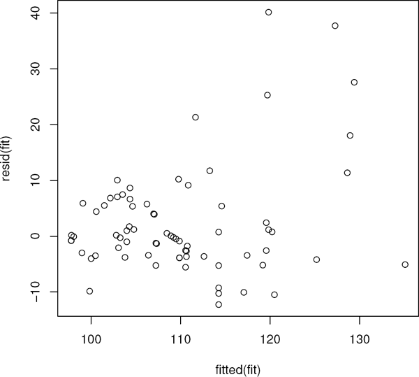
Example 4.7.2 (Sine Cosine Model).

For this example we generated n = 197 observations from the model

$\begin{array}{cc}{y}_i=5\sin (3x)+6\cos \left(x/4\right)+e_i,& (4.29)\end{array}$

where ei are N(0, 100) variates and xi goes from 1 to 50 in increments of 0.25. The data are in the set sincos. The appropriate sm function is sm.regression. It has an argument h for bandwidth, but if this is omitted a data-driven bandwidth is used. The fit is obtained as shown in the following code segment (the vectors x and y contain the data). The default kernel is the normal pdf and the option display=“none” turns off the automatic plot. Figure 4.8 displays the data and the fit.

> library(sm)

> fit <- sm.regression(x,y,display=“none”)

> fit$h   ## Data driven bandwidth

[1] 4.211251

> plot(y˜ x,xlab=expression(x),ylab=expression(y))

> with(fit,lines(estimate˜ eval.points))

> title(“sm.regression Fit of Sine-Cosine Data”)

Note that the procedure estimated the bandwidth to be 4.211.

The smoother sm.regression is not robust. As an illustration, consider the sine-cosine data of Example 4.7.2. We modified the data by replacing y187 with the outlying value of 800. As shown in Figure 4.9, the sm.regression fit (solid line) of the modified data is severely impaired in the neighborhood of the outlier. The valley at x = 36 has essentially been missed by the fit. For ease of comparison, we have also displayed the sm.regression fit on the original data (broken line), which finds this valley.

A smoother which has robust capabilities is loess which was developed by Cleveland et al. (1992). This is a base R routine. Briefly, loess smooths at a point xi via a local linear fit. The percentage of data used for the local fit is the analogue of the bandwidth parameter. The default percentage is 75%, but it can be changed by using the argument span. Also, by default, the local fitting procedure is based on a weighted least squares procedure. As shown by the broken line fit in Figure 4.10, for the modified sine-cosine data, loess is affected in the same way as the sm fit; i.e., it has missed the valley at x = 36. Setting the argument family=“symmetric” in the call to loess, though, invokes a robust local linear model fit. This is the solid line in Figure 4.10 which is very close to the sm fit based on the original data. Exercise 4.9.18 asks the reader to create a similar graphic. The following code segment generates Figure 4.10; the figure demonstrates the importance in obtaining a robust fit in addition to a traditional fit. We close this section with two examples using real datasets.

Example 4.7.3 (Old Faithful).

This dataset concerns the eruptions of Old Faithful, which is a geyser in Yellowstone National Park, Wyoming. The dataset is faithful in base R. As independent and dependent variables, we chose respectively the duration of the eruption and the waiting time between eruptions. In the top panel of Figure 4.11 we display the data overlaid with the loess fit. There is an increasing trend, i.e., longer eruption times lead to longer waiting times between eruptions. There appear to be two groups in the plot based on lower or higher duration of eruption times. As the residual plot shows, the loess fit has detrended the data.

Example 4.7.4 (Maximum January Temperatures in Kalamazoo).

The dataset weather contains weather data for the month of January for Kalamazoo, Michigan, from 1900 to 1995. For this example, our response variable is avemax which is the average maximum temperature in January. The top panel of Figure 4.12 shows the response variable over time. There seems to be little trend in the data. The lower panel shows the loess fits, local LS (solid line) and local robust (broken line). The fits are about the same. They do show a slight pattern of a warming trend between 1930 and 1950.

4.8 Correlation

In a simple linear regression problem involving a response variable Y and a predictor variable X, the fit of the model is of main interest. In particular, we are often interested in predicting the random variable Y in terms of x and we treat x as nonstochastic. In certain settings, though, the pair (X, Y) is taken to be a random vector and we are interested in measuring the strength of a relationship or association between the random variables X and Y. By no association, we generally mean that the random variables X and Y are independent, so the basic hypotheses of interest in this section are:

$\begin{array}{cc}{H}_0:X\text{and}Y\text{are independent versus}{H}_A:X\text{and}Y\text{are dependent}.& (4.30)\end{array}$

For this section, assume that (X, Y) is a continuous random vector with joint cdf and pdf F(x,y) and f(x,y), respectively. Recall that X and Y are independent random variables if their joint cdf factors into the product of the marginal cdfs; i.e., F(x,y) = FX(x)FY(y) where FX(x) and FY(y) are the marginal cdfs of X and Y, respectively. In Section 2.7 we discussed a χ2 goodness-of-fit test for independence when X and Y are discrete random variables. For the discrete case, independence is equivalent to the statement P(X = x,Y = y) = P(X = x)P(Y = y) for all x and y. In fact, the null expected frequencies of the χ2 goodness-of-fit test statistic are based on this statement.2 In the continuous case, we consider measures of association between X and Y. We discuss the traditional Pearson’s measure of association (the correlation coefficient ρ) and two popular nonparametric measures (Kendall’s τK and Spearman’s ρS).

Let (X1, Y1), (X2, Y2),..., (Xn, Yn) denote a random sample of size n on the random vector (X,Y). Using this notation, we discuss the estimation, associated inference, and R computation for these measures. Our discussion is brief and many of the facts that we state are discussed in detail in most introductory mathematical statistics texts; see, for example, Chapters 9 and 10 of Hogg et al. (2013).

4.8.1 Pearson’s Correlation Coefficient

The traditional correlation coefficient between X and Y is the ratio of the covariance between X and Y to the product of their standard deviations, i.e.,

$\begin{array}{cc}\rho =\frac{E[(X-{\mu }_X)(Y-{\mu }_Y)]}{{\sigma }_X{\sigma }_Y},& (4.31)\end{array}$

where μX, σX and μY, σY are the respective means and standard deviations of X and Y. The parameter ρ requires, of course, the assumption of finite variance for both X and Y. It is a measure of linear association between X and Y. It can be shown that it satisfies the properties: −1 ≤ ρ ≤ 1; ρ = ±1 if and only if Y is a linear function of X (with probability 1); and ρ > (<) 0 is associated with a positive (negative) linear relationship between Y and X. Note that if X and Y are independent then ρ = 0. In general, the converse is not true. The contrapositive, though, is true; i.e., $\rho \ne 0\Rightarrow X$ and Y are dependent.

Usually ρ is estimated by the nonparametric estimator. The numerator is estimated by the sample covariance, $n^{-1}{\sum }_{i=1}^n\left(X_i-\overline{X}\right)\left(Y_i-\overline{Y}\right)$, while the denominator is estimated by the product of the sample standard deviations (with n, not n – 1, as divisors of the sample variances). This simplifies to the sample correlation coefficient given by

$\begin{array}{cc}r=\frac{{\displaystyle {\sum }_{i=1}^n\left(X_i-\overline{X}\right)\left(Y_i-\overline{Y}\right)}}{\sqrt{{\displaystyle {\sum }_{i=1}^n{\left(X_i-\overline{X}\right)}^2\cdot {\displaystyle {\sum }_{i=1}^n{\left(Y_i-\overline{Y}\right)}^2}}}}.& (4.32)\end{array}$

Similarly, it can be shown that r satisfies the properties: −1 ≤ r ≤ 1; r = ±1 if there is a deterministic linear relationship for the sample (Xi, Yi); and r > (<)0 is associated with a positive (negative) linear relationship between Yi and Xi. The estimate of the correlation coefficient is directly related to simple least squares regression. Let ${\widehat{\sigma }}_x$ and ${\widehat{\sigma }}_y$ denote the respective sample standard deviations of X and Y. Then we have the relationship

$\begin{array}{cc}r=\frac{{\widehat{\sigma }}_x}{{\widehat{\sigma }}_y}\widehat{\beta },& (4.33)\end{array}$

where $\widehat{\beta }$ is the least squares estimate of the slope in the simple regression of Yi on Xi. It can be shown that, under the null hypothesis, $\sqrt{n}r$ is asymptotically N(0,1). Inference for ρ can be based on this asymptotic result, but usually the t-approximation discussed next is used.

If we make the much stronger assumption that the random vector (X, Y) has a bivariate normal distribution, then the estimator r is the maximum likelihood estimate (MLE) of ρ. Based on expression (4.33) and the usual t-ratio in regression, under H0, the statistic

$\begin{array}{cc}t=\frac{\sqrt{n-2}r}{\sqrt{1-r^2}}& (4.34)\end{array}$

has t-distribution with n – 2 degrees of freedom; see page 508 of Hogg et al. (2013). Thus a level α test of the hypotheses (4.30) is to reject H0 in favor of HA if $\left|t\right|>t_{\alpha /2,n-2}$. Furthermore, for general ρ, it can be shown that log[(1+r)/(1–r)] is approximately normal with mean log[(1+ρ)/(1–ρ)]. Based on this, approximate confidence intervals for ρ can be constructed. In practice, usually the strong assumption of bivariate normality cannot be made. In this case, the t-test and confidence interval are approximate. For computation in R, assume that the R vectors x and y contain the samples X1, ..., Xn and Y1,...,Yn, respectively. Then the R function cor. test computes this analysis; see Example 4.8.1 below. If inference is not needed the function cor may be used to just obtain the estimate.

4.8.2 Kendall’s τK

Kendall’s τK is the first nonparametric measure of association that we discuss. As above, let (X, Y) denote a jointly continuous random vector. Kendall’s τK is a measure of monotonicity between X and Y. Let the two pairs of random variables (X1,Y1) and (X2,Y2) be independent random vectors with the same distribution as (X,Y). We say that the pairs (X1,Y1) and (X2,Y2) are concordant or discordant if

$\text{sign}\{(X_1-X_2)(Y_1-Y_2)\}=1\text{or sign}\{(X_1-X_2)(Y_1-Y_2)\}=-1,$

respectively. Concordant pairs are indicative of increasing monotonicity between X and Y, while discordant pairs indicate decreasing monotonicity. Kendall’s τK measures this monotonicity in a probability sense. It is defined by

$\begin{array}{cc}{\tau }_K=P[\text{sign}\{(X_1-X_2)(Y_1-Y_2)\}=1]-P[\text{sign}\{(X_1-X_2)(Y_1-Y_2)\}=-1].& (4.35)\end{array}$

It can be shown that −1 ≤ τK ≤ 1; τK > 0 indicates increasing monotonicity; τK < 0 indicates decreasing monotonicity; and τK = 0 reflects neither monotonicity. It follows that if X and Y are independent then τK = 0. While the converse is not true, the contrapositive is true; i.e., ${\tau }_K\ne 0\Rightarrow X$ and Y are dependent.

Using the random sample (X1, Y1), (X2, Y2),..., (Xn, Yn), a straightforward estimate of τK is simply to count the number of concordant pairs in the sample and subtract from that the number of discordant pairs. Standardization of this statistic leads to

$\begin{array}{cc}{\widehat{\tau }}_K={\left(\begin{array}{c}n\\ 2\end{array}\right)}^{-1}{\displaystyle \sum _{i<j}\text{sign}\{(X_i-X_j)(Y_i-Y_j)\}}& (4.36)\end{array}$

as our estimate of τK. Since the statistic ${\widehat{\tau }}_K$ is a Kendall’s τK based on the empirical sample distribution, it shares the same properties; i.e., ${\widehat{\tau }}_K$ is between −1 and 1; positive values of ${\widehat{\tau }}_K$ reflect increasing monotonicity; and negative values reflect decreasing monotonicity. It can be shown that ${\widehat{\tau }}_K$is an unbiased estimate of τK. Further, under the assumption that X and Y are independent, the statistic ${\widehat{\tau }}_K$ is distribution-free with mean 0 and variance 2(2n + 5)/[9n(n − 1)]. Tests of the hypotheses (4.30) can be based on the exact finite sample distribution. Tie corrections for the test are available. Furthermore, distribution-free confidence intervals3 for τK exist. R computation of the inference for Kendall’s τK is obtained by the function cor.test with method=“kendall”; see Example 4.8.1. Although this R function does not compute a confidence interval for τK, in Section 4.8.4 we provide an R function to compute the percentile bootstrap confidence interval for τK.

4.8.3 Spearman’s ρs

In defining Spearman’s ρS, it is easier to begin with its estimator. Consider the random sample (X1,Y1),(X2,Y2),..., (Xn,Yn). Denote by R(Xi) the rank of Xi among X1, X2,..., Xn and likewise define R(Yi) as the rank of Yi among Y1, Y2,..., Yn. The estimate of ρS is simply the sample correlation coefficient with Xi and Yi replaced respectively by R(Xi) and R(Yi). Let rS denote this correlation coefficient. Note that the denominator of rS is a constant and that the sample mean of the ranks is (n + 1)/2. Simplification leads to the formula

$\begin{array}{cc}{r}_S=\frac{{\displaystyle {\sum }_{i=1}^n(R(X_i)-[(n+1)/2])(R(Y_i)-[(n+1)/2])}}{n(n^2-1)/12}.& (4.37)\end{array}$

This statistic is a correlation coefficient, so it is between ±1, It is ±1 if there is a strictly increasing (decreasing) relation between Xi and Yi; hence, similar to Kendall’s ${\widehat{\tau }}_K$, it estimates monotonicity between the samples. It can be shown that

$E\left(r_S\right)=\frac{3}{n+1}[{\tau }_K+(n-2)(2\gamma -1)],$

where γ = P[(X2 - X1)(Y3 - Y1) > 0]. The parameter that rS is estimating is not as easy to interpret as the parameter τK.

If X and Y are independent, it follows that rS is a distribution-free statistic with mean 0 and variance (n − 1)-1. We accept HA : X and Y are dependent for large values of |rS|. This test can be carried out using the exact distribution or approximated using the z-statistic $\sqrt{n-1}{r}_S$. In applications, however, similar to expression (4.34), the t-approximation4 is often used, where

$\begin{array}{cc}t=\frac{\sqrt{n-2}{r}_S}{\sqrt{1-r_S^2}}.& (4.38)\end{array}$

There are distribution-free confidence intervals for ρS and tie corrections5 are available. The R command cor.test with method=“spearman” returns the analysis based on Spearman’s rS. This computes the test statistic and the p-value, but not a confidence interval for ρS. Although the parameter ρS is difficult to interpret, nevertheless confidence intervals are important for they give a sense of the strength (effect size) of the estimate. As with Kendall’s τK, in Section 4.8.4, we provide an R function to compute the percentile bootstrap confidence interval for ρS.

Remark 4.8.1 (Hypothesis Testing for Associations).

In general, let ρG denote any of the measures of association discussed in this section. If ρG ≠ 0 then X and Y are dependent. Hence, if the statistical test rejects ρG = 0, then we can statistically accept HA that X and Y are dependent. On the other hand, if ρG = 0, then X and Y are not necessarily independent. Hence, if the test fails to accept HA, then we should not conclude independence between X and Y. In this case, we should conclude that there is not significant evidence to refute ρG = 0.

4.8.4 Computation and Examples

We illustrate the R function cor.test in the following example.

Example 4.8.1 (Baseball Data, 2010 Season).

Datasets of major league baseball statistics can be downloaded at the site baseballguru.com. For this example, we investigate the relationship between the batting average of a full-time player and the number of home runs that he hits. By full-time we mean that the batter had at least 450 official at bats during the season. These data are in the npsm dataset bb2010. Figure 4.13 displays the scatterplot of home run production versus batting average for full-time players. Based on this plot there is an increasing monotone relationship between batting average and home run production, although the relationship is not very strong.

In the next code segment, the R analyses (based on cor.test) of Pearson’s, Spearman’s, and Kendall’s measures of association are displayed.

> with(bb2010,cor.test(ave,hr))

   Pearson’s product-moment correlation

data: ave and hr

t = 2.2719, df = 120, p-value = 0.02487

alternative hypothesis: true correlation is not equal to 0

95 percent confidence interval:

 0.02625972 0.36756513

sample estimates:

  cor

0.2030727

> with(bb2010,cor.test(ave,hr,method=“spearman”))

   Spearman’s rank correlation rho

data: ave and hr

S = 234500, p-value = 0.01267

alternative hypothesis: true rho is not equal to 0

sample estimates:

  rho

0.2251035

> with(bb2010,cor.test(ave,hr,method=“kendall”))

   Kendall’s rank correlation tau

data: ave and hr

z = 2.5319, p-value = 0.01134

alternative hypothesis: true tau is not equal to 0

sample estimates:

  tau

0.1578534

For each of the methods the output contains a test statistic and associated p-value as well as the point estimate of the measure of association. Pearson’s also contains the estimated confidence interval (95% by default). For example the results from Pearson’s analysis give r = 0.203 and a p-value of 0.025. While all three methods show a significant positive association between home run production and batting average, the results for Spearman’s and Kendall’s procedures are somewhat stronger than that of Pearson’s. Based on the scatterplot, Figure 4.13, there are several outliers in the dataset which may have impaired Pearson’s r. On the other hand, Spearman’s rS and Kendall’s ${\widehat{\tau }}_K$ are robust to the effects of the outliers.

The output for Spearman’s method results in the value of rS and the p-value of the test. It also computes the statistic

$S={\displaystyle \sum _{i=1}^n{[R(X_i)-R(Y_i)]}^2}.$

Although it can be shown that

$r_S=1-\frac{6S}{n^2-n};$

the statistic S does not readily show the strength of the association, let alone the sign of the monotonicity. Hence, in addition, we advocate forming the z statistic or the t-approximation of expression (4.38). The latter gives the value of 2.53 with an approximate p-value of 0.0127. This p-value agrees with the p-value calculated by cor. test and the value of the standardized test statistic is readily interpreted. See Exercise 4.9.16.

As with the R output for Spearman’s procedure, the output for Kendall’s procedure includes ${\widehat{\tau }}_K$ and the p-value of the associated test. The results of the analysis based on Kendall’s procedure indicate that there is a significant monotone increasing relationship between batting average and home run production, similar to the results for Spearman’s procedure. The estimate of association is smaller than that of Spearman’s, but recall that they are estimating different parameters. Instead of a z-test statistic, R computes the test statistic T which is the number of pairs which are monotonically increasing. It is related to ${\widehat{\tau }}_K$ by the expression

$T=\left\{\left(\begin{array}{c}n\\ 2\end{array}\right)[1+{\widehat{\tau }}_K]\right\}/2.$

The statistic T does not lend itself easily to interpretation of the test. Even the sign of monotonicity is missing. As with the Spearman’s procedure, we recommend also computing the standardized test statistic; see Exercise 4.9.17.

In general, a confidence interval yields a sense of the strength of the relationship. For example, a “quick” standard error is the length of a 95% confidence interval divided by 4. The function cor.test does not compute confidence intervals for Spearman’s and Kendall’s methods. We have written an R function, cor. boot. ci, which obtains a percentile bootstrap confidence interval for each of the three measures of association discussed in this section. Let B = [X, Y] be the matrix with the samples of Xi’s in the first column and the samples of Yi’s in the second column. Then the bootstrap scheme resamples the rows of B with replacement to obtain a bootstrap sample of size n. This is performed nBS times. For each bootstrap sample, the estimate of the measure of association is obtained. These bootstrap estimates are collected and the α/2 and (1 - α/2) percentiles of this collection form the confidence interval. The default arguments of the function are:

> args(cor.boot.ci)

function (x, y, method = “spearman”, conf = 0.95, nbs = 3000)

NULL

Besides Spearman’s procedure, bootstrap percentile confidence intervals are computed for ρ and τK by using respectively the arguments method=“pearson” and method=“kendall”. Note that (1 - α) is the confidence level and the default number of bootstrap samples is set at 3000. We illustrate this function in the next example.

Example 4.8.2 (Continuation of Example 4.8.1).

The code segment below obtains a 95% percentile bootstrap confidence interval for Spearman’s ρS.

> library(boot)

> with(bb2010,cor.boot.ci(ave,hr))

  2. 5% 97. 5%

0.05020961 0.39888150

The following code segment computes percentile bootstrap confidence intervals for Pearson’s and Kendall’s methods.

> with(bb2010,cor.boot.ci(ave,hr,method=‘pearson’))

  2. 5%  97. 5%

0.005060283 0.400104126

> with(bb2010, cor. boot. ci (ave,hr,method= ‘kendall ’))

  2. 5%  97. 5%

0.02816001 0.28729659

To show the robustness of Spearman’s and Kendall’s procedures, we changed the home run production of the 87th batter from 32 to 320; i.e., a typographical error. Table 4.1 compares the results for all three procedures on the original and changed data.6

Note that the results for Spearman’s and Kendall’s procedures are essentially the same on the original dataset and the dataset with the outlier. For Pearson’s procedure, though, the estimate changes from 0.20 to 0.11. Also, the confidence interval has been affected.

4.9 Exercises

1. 4.9.1. Obtain a scatterplot of the telephone data. Overlay the least squares and R fits.
2. 4.9.2. Write an R function which given the results of a call to rfit returns the diagnostic plots: Studentized residuals versus fitted values, with ±2 horizontal lines for outlier identification; normal q – q plot of the Studentized residuals, with ±2 horizontal lines outliers for outlier identification; histogram of residuals; and a boxplot of the residuals.

3. 4.9.3. Consider the free fatty acid data.

   1. (a) For the Wilcoxon fit, obtain the Studentized residual plot and q–q plot of the Studentized residuals. Comment on the skewness of the errors.
   2. (b) Redo the analysis of the free fatty acid data using the bent scores (bentscores 1). Compare the summary of the regression coefficients with those from the Wilcoxon fit. Why is the bent score fit more precise (smaller standard errors) than the Wilcoxon fit?
4. 4.9.4. Using the baseball data, calculate a large sample confidence interval for the slope parameter when regressing weight on height. Compare the results to those obtained using the bootstrap discussed in Section 4.6.

5. 4.9.5. Consider the following data:

   x	1	2	3	4	5	6	7	8	9	10	11	12	13	14	15
   y	-7	0	5	9	-3	-6	18	8	-9	-20	-11	4	-1	7	5

   Consider the simple regression model: Y = β0 + β1x + e.

   1. (a) For Wilcoxon scores, write R code which obtains a sensitivity curve of the rfit of the estimate of β1, where the sensitivity curve is the difference in the estimates of β1 between perturbed data and the original data.
   2. (b) For this exercise, use the above data as the original data. Let ${\widehat{\beta }}_1$ denote the Wilcoxon estimate of slope based on the original data. Then obtain 9 perturbed datasets using the following sequence of replacements to y15: −995, −95, −25, −5, 5,10, 30,100,1000. Let ${\widehat{\beta }}_1{}_j$ be the Wilcoxon fit of the jth perturbed dataset for j = 1, 2,..., 9. Obtain the sensitivity curve which is the plot of ${\widehat{\beta }}_1{}_j-{\widehat{\beta }}_1$ versus the jth replacement value for y15.
   3. (c) Obtain the sensitivity curve for the LS fit. Compare it with the Wilcoxon sensitivity curve.

6. 4.9.6. For the simple regression model, the estimator of slope proposed by Theil (1950) is defined as the median of the pairwise slopes:

   ${\widehat{\beta }}_T=\text{med}\left\{b_{ij}\right\}$

   where bij = (yj - yi)/(xj - xi) for i < j.

   1. (a) Write an R function which takes as input a vector of response variables and a vector of explanatory variables and returns the Theil estimate.
   2. (b) For a simple regression model where the predictor is a continuous variable, write an R function which computes the bootstrap percentile confidence interval for the slope parameter based on Theil’s estimate.
   3. (c) Show that Theil’s estimate reduces to the the Hodges-Lehmann estimator for the two-sample location problem.

7. 4.9.7. Consider the data of Example 4.4.1.

   1. (a) Obtain a scatterplot of the data.
   2. (b) Obtain the Wilcoxon fit of the linear trend model. Overlay the fit on the scatterplot. Obtain the Studentized residual plot and normal q–q plots. Identify any outliers and comment on the quality of fit.
   3. (c) Obtain a 95% confidence interval for the slope parameter and use it to test the hypothesis of 0 slope.
   4. (d) Estimate the mean of the response when time has the value 16 and find the 95% confidence interval for it which was discussed in Section 4.4.4.

8. 4.9.8. Bowerman et al. (2005) present a dataset concerning the value of a home (x) and the upkeep expenditure (y). The data are in qhic. The variable x is in $1000’s of dollars while the y variable is in $10’s of dollars.

   1. (a) Obtain a scatterplot of the data.
   2. (b) Use Wilcoxon Studentized residual plots, values of $\widehat{\tau }$, and values of the robust R2 to decide whether a linear or a quadratic model fits the data better.
   3. (c) Based on your model, estimate the expected expenditures (with a 95% confidence interval) for a house that is worth $155,000.
   4. (d) Repeat (c) for a house worth $250,000.
9. 4.9.9. Rewrite the aligned.test function to take an additional design matrix as its third argument instead of group/treatment membership. That is, for the model Y = α1 + X1β1 + X2β2 + e, test the hypothesis H0 : β2 = 0.

10. 4.9.10. Hettmansperger and McKean (2011) discuss a dataset in which the dependent variable is the cloud point of a liquid, a measure of degree of crystallization in a stock, and the independent variable is the percentage of I-8 in the base stock. For the readers’ convenience, the data can be found in the dataset cloud in the package npsm.

    1. (a) Scatterplot the data. Based on the plot, is a simple linear regression model appropriate?
    2. (b) Show by residual plots of the fits that the linear and quadratic polynomials are not appropriate but that the cubic model is.
    3. (c) Use the R function polydeg, with a super degree set at 5, to determine the degree of the polynomial. Compare with Part (b).

11. 4.9.11. Devore (2012) discusses a dataset on energy. The response variable is the energy output in watts while the independent variable is the temperature difference in degrees K. A polynomial fit is suggested. The data are in the dataset energy.

    1. (a) Scatterplot the data. What degree of polynomial seems suitable?
    2. (b) Use the R function polydeg, with a super degree set at 6, to determine the degree of the polynomial.
    3. (c) Based on a residual analysis, does the polynomial fit of Part (b) provide a good fit?

12. 4.9.12. Consider the weather dataset, weather, discussed in Example 4.7.4. One of the variables is mean average temperature for the month of January (meantmp).

    1. (a) Obtain a scatterplot of the mean average temperature versus the year. Determine the warmest and coldest years.
    2. (b) Obtain the loess fit of the data. Discuss the fit in terms of years, (were there warm trends, cold trends?).

13. 4.9.13. As in the last problem, consider the weather dataset, weather. One of the variables is total snowfall (in inches), totalsnow, for the month of January.

    1. (a) Scatterplot total snowfall versus year. Determine the years of maximal and minimal snowfalls.
    2. (b) Obtain the local LS and robust loess fits of the data. Compare the fits.
    3. (c) Perform a residual analysis on the robust fit.
    4. (d) Obtain a boxplot of the residuals found in Part (c). Identify the outliers by year.
14. 4.9.14. In the discussion of Figure 4.7, the nonparametric regression fit by ksmooth detects an artificial valley. Obtain the locally robust loess fit of this dataset (poly) and compare it with the ksmooth fit.
15. 4.9.15. Using the baseball data, obtain the scatterplot between the variables home run productions and RBIs. Then compute the Pearson’s, Spearman’s, and Kendall’s analyses for these variables. Comment on the plot and analyses.
16. 4.9.16. Write an R function which computes the t-test version of Spearman’s procedure and returns it along with the corresponding p-value and the estimate of ρS.
17. 4.9.17. Repeat Exercise 4.9.16 for Kendall’s procedure.
18. 4.9.18. Create a graphic similar to Figure 4.10.

19. 4.9.19. Recall that, in general, the three measures of association estimate different parameters. Consider bivariate data (Xi,Yi) generated as follows:

    $Y_i=X_i+e_i,i=1,2,...,n,$

    where Xi has a standard Laplace (double exponential) distribution, ei has a standard N(0,1) distribution, and Xi and ei are independent.

    1. (a) Write an R script which generates this bivariate data. The supplied R function rlaplace(n) generates n iid Laplace variates. For n = 30, compute such a bivariate sample. Then obtain the scatterplot and the association analyses based on the Pearson’s, Spearman’s, and Kendall’s procedures.
    2. (b) Next write an R script which simulates the generation of these bivariate samples and collects the three estimates of association. Run this script for 10,000 simulations and obtain the sample averages of these estimates, their corresponding standard errors, and approximate 95% confidence intervals. Comment on the results.

20. 4.9.20. The electronic memory game Simon was first introduced in the late 1970s. In the game there are four colored buttons which light up and produce a musical note. The device plays a sequence of light/note combinations and the goal is to play the sequence back by pressing the buttons. The game starts with one light/note and progressively adds one each time the player correctly recalls the sequence.7

    Suppose the game were played by a set of statistics students in two classes (time slots). Each student played the game twice and recorded his or her longest sequence. The results are in the dataset simon.

    Regression toward the mean is the phenomenon that if an observation is extreme on the first trial it will be closer to the average on the second trial. In other words, students that scored higher than average on the first trial would tend to score lower on the second trial and students who scored low on the first trial would tend to score higher on the second.

    1. (a) Obtain a scatterplot of the data.
    2. (b) Overlay an R fit of the data. Use Wilcoxon scores. Also overlay the line y = x.
    3. (c) Obtain an R estimate of the slope of the regression line as well as an associated confidence interval.
    4. (d) Do these data suggest a regression toward the mean effect?

1 See Section 3.5 of Hettmansperger and McKean (2011).

2 For the continuous case, this statement is simply 0 = 0, so the χ2 goodness-of-fit test is not an option.

3 See Chapter 8 of Hollander and Wolfe (1999).

4 See, for example, page 347 of Huitema (2011).

5 See Hollander and Wolfe (1999).

6 These analyses were run in a separate step so they may differ slightly from those already reported.

7 The game is implemented on the web. The reader is encouraged to use his or her favorite search engine and try it out.