Chapter 3. Programming Tools for OpenACC
Robert Dietrich, Technische Universität Dresden Sameer Shende, ParaTools/University of Oregon
Software tools can significantly improve the application development process. With the spread of GPU-accelerated systems and OpenACC programs, a variety of development tools are now available, including code editors, compilers, debuggers, and performance analysis tools.
A proper code editor with syntax highlighting or an integrated development environment (IDE) helps spot syntax errors. Compilers print error messages in case of nonconforming or erroneous source code. Typically, they also provide the option to print additional information on the compilation process, such as the implementation of OpenACC directives. However, several types of errors occur during the execution of the binary. Debuggers provide the means to dynamically track errors in the program at run time. When programming models, such as OpenACC, are used to accelerate an application, the performance of the program should be investigated and tuned with the help of performance analysis tools.
3.1 Common Characteristics of Architectures
The OpenACC programming model has been developed for many core devices, such as GPUs. It targets host-directed execution using an attached or integrated accelerator. This means that the host is executing the main program and controls the activity of the accelerator. To benefit from OpenACC directives, the executing devices should provide parallel computing capabilities that can be addressed with at least one of the three levels of parallelism: gang, worker, or vector.
OpenACC accelerator devices typically provide capabilities for efficient vector processing, such as warps for CUDA devices, wavefronts on AMD GPUs, and 512-bit SIMD (single-instruction, multiple-data) units on Intel Xeon Phi. The architecture of Intel MIC (Many Integrated Core) devices works well with multithreading and thus worker parallelism. GPUs are typically split into clusters of ALUs (arithmetic logic units), such as NVIDIA SMs (streaming multiprocessors), which maps to gang parallelism. Thus, the device capabilities should match the values of the OpenACC vector, worker, and gang size. Performance tools that use the OpenACC 2.5 profiling interface can acquire this information for a compute kernel in the respective enqueue operation, because these values are fixed per compute kernel.
OpenACC uses the concept of computation offloading. This allows you to execute computationally intensive work, or workloads that simply fit to the architecture of an accelerator, on an offloading device. This means that OpenACC devices are most often host-controlled and not self-hosted. Nevertheless, some OpenACC compilers (e.g., PGI’s multicore back end) generate code for multicore CPUs from OpenACC directives.
In terms of performance analysis, computation offloading requires that you capture information on the host and device execution, and a correlation must be established between host and device data. Performance measurement on host processors can provide fine-grained data, whereas accelerator data typically are not more detailed than up to the task level, such as start and end of compute kernels and data transfers. Transfer times can determine the bandwidth of a data movement.
In general, acquisition of device-side performance data depends on the accelerator and respective APIs to access them. For example, a device-specific API may provide access to hardware counters, such as cache accesses or IPCs (instructions per cycle).
3.2 Compiling OpenACC Code
OpenACC builds on top of the programming languages C, C++, and Fortran. Therefore, OpenACC programs are compiled similarly to other programs written in one of these three languages. Because of the nature of compiler directives, every compiler for these languages can compile a program that contains OpenACC directives. Compilers can simply ignore directives, as it does comments. A compiler with OpenACC support is needed when OpenACC runtime library routines are used. Keep this in mind if you intend to also run the code without OpenACC.
Compilers with support for the OpenACC API typically provide a switch that enables the interpretation of OpenACC directives (for example, -acc for the PGI compiler, and –fopenacc for the GNU compiler). This usually includes the header openacc.h automatically, as well as a link to the compiler’s OpenACC runtime library. Because OpenACC has been developed for performance portable programming, there is typically a compiler option to specify the target architecture. The default target might fit a variety of devices, but most often it does not provide the best performance. Table 3.1 shows an overview of OpenACC compiler flags for several known OpenACC compilers.
Table 3.1 Compiler flags for various OpenACC compilers
COMPILER |
COMPILER FLAGS |
ADDITIONAL FLAGS |
PGI |
|
|
GCC |
|
|
OpenUH |
Compile: Link: |
|
Cray |
C/C++: Fortran: |
|
An example of a complete compile command and the compiler output are given in Listing 3.1 for the PGI C compiler. It generates an executable prog for the OpenACC program prog.c. The switch –ta=tesla:kepler optimizes the device code for NVIDIA’s Kepler architecture. The flag –Minfo=accel prints additional information on the implementation of OpenACC directives and clauses.
Listing 3.1 Exemplary PGI compiler output with -Minfo=accel for a simple OpenACC reduction
pgcc –acc –ta=nvidia:kepler –Minfo=accel prog.c –o prog
reduceAddOpenACC_kernel:
40, Generating implicit copyin(data[1:size-1])
41, Loop is parallelizable
Accelerator kernel generated
Generating Tesla code
41, #pragma acc loop gang, vector(128)
/* blockIdx.x threadIdx.x */
42, Generating implicit reduction(+:sum)
The number of compilers with OpenACC support1 has grown over time. PGI and Cray are commercial compilers. PGI also provides a community edition without license costs. Among the open source compilers are the GCC2 and several OpenACC research compilers, such as Omni from the University of Tsukuba,3 OpenARC from Oak Ridge National Laboratory,4 and OpenUH from the University of Houston.5
1. http://www.openacc.org/content/tools.
2. https://gcc.gnu.org/wiki/OpenACC.
4. http://ft.ornl.gov/research/openarc.
5. https://you.stonybrook.edu/exascallab/downloads/openuh-compiler/..
3.3 Performance Analysis of OpenACC Applications
OpenACC is about performance. It provides the means to describe parallelism in your code. However, the compiler and the OpenACC runtime implement this parallelism. Furthermore, many execution details are implicitly hidden in the programming model. Performance analysis tools can expose those implicit operations and let you investigate the runtime behavior of OpenACC programs. You can gain insight into execution details, such as IO (input/output) and memory operations as well as host and device activities.
There is a variety of performance-relevant information that helps you understand the runtime behavior of an application. For small OpenACC programs that run on a single node, it might be enough to use simple profiling options, such as the PGI_ACC_TIME environment variable. Setting it to 1 prints profiling output to the console. However, this variable is available only with the PGI OpenACC implementation. Other compilers provide similar options.
To analyze complex programs, a performance tool should support all paradigms and programming models used in the application, because inefficiency might arise from their interaction. Depending on the tool, three levels of parallelism can be covered: process parallelization, multithreading, and offloading. OpenACC refers to the latter, but offloading is often used in combination with Message Passing Interface (MPI) for interprocess communication, and with OpenMP for multithreading. When a specific region has been exposed for optimization, hardware counters might help identify more fine-grained performance issues.
Performance analysis is obviously useful for tuning programs and should be a part of a reasonable application development cycle. It starts with the measurement preparation, followed by the measurement run and the analysis of the performance data, and concludes with code optimization. In the following, we focus on the first three steps.
During measurement preparation you select and configure data sources, which will provide information on program execution. It does not require changing the application code in every case (see the following section). The measurement itself is an execution run while performance data are recorded. The measurement data are then analyzed, often with the help of performance tools. Based on the performance analysis results you try to optimize the code, and then you repeat the whole process.
Optimizations or code changes might not always result in better performance. Comparing different execution runs helps you understand the impact of code changes or evaluate the application’s performance on different platforms and target devices. Several tools are available that enable such performance comparisons (for example, TAU6 and Vampir7).
6. Sameer Shende and Allen D. Malony, “The TAU Parallel Performance System,” International Journal of High Performance Computing Applications, 20(2) (2006): 287–311. http://tau.uoregon.edu.
7. Andreas Knüpfer et al., “The Vampir Performance Analysis Tool-Set,” Tools for High Performance Computing (2008): 139–155.
3.3.1 Performance Analysis Layers and Terminology
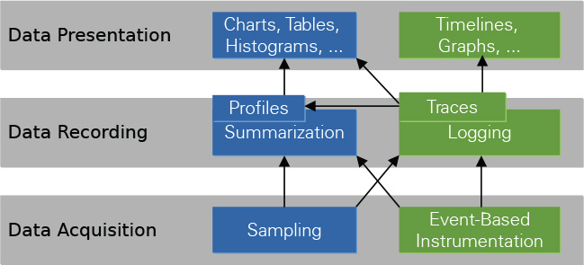
The goal of performance analysis is the detection of bottlenecks and inefficiencies in the execution of a program to support application developers in tuning. As depicted in Figure 3.1, there are three analysis layers: data acquisition, data recording, and data presentation. Performance tools typically implement all layers and try to hide the complexity of the analysis process from the user. For a better understanding of the analysis results and a clarification of terminology, analysis layers and techniques are discussed next.
Note: Compare to Thomas Ilsche, Joseph Schuchart, Robert Schöne, and Daniel Hackenberg, “Combining Instrumentation and Sampling for Trace-Based Application Performance Analysis,” Tools for High Performance Computing (2014): 123–136.
3.3.2 Performance Data Acquisition
There are two fundamental approaches to acquire data during the program run.
• Sampling is a “pull” mechanism, which queries information on what the application is doing. The rate of such queries (samples) can be set to a fixed value, resulting in a constant and predictable runtime perturbation. However, the measurement accuracy depends on the sampling frequency. A low sampling frequency might miss valuable information; a high sampling frequency might introduce too much overhead. Also, timer-based interrupts generate a constant sampling rate, whereas other interrupt generators, such as counter overflow, might not provide samples at regular intervals.
• Event-based instrumentation typically modifies the application to “push” information about its activity to the performance measurement infrastructure. Instrumentation can be placed anywhere in the code to mark, for instance, begin and end of program functions, library calls, and code regions. All instrumented events must be executed to be observed and thus will reflect how the program behaved. Because the event rate is unknown at compile time, the runtime perturbation cannot be predicted and can be of several orders of magnitude in a worst-case scenario. Advantages and drawbacks of both approaches have been discussed in literature—for example, by Ilsche et al.8
8. Thomas Ilsche, Joseph Schuchart, Robert Schöne, and Daniel Hackenberg, “Combining Instrumentation and Sampling for Trace-Based Application Performance Analysis,” Tools for High Performance Computing (2014): 123–136.
Since OpenACC 2.5, the specification describes a profiling interface that enables you to record OpenACC events during the execution of an OpenACC program. It is described in Section 3.3.4. Interfaces can be used for data acquisition for many other programming models, such as CUPTI for CUDA,9 OMPT for OpenMP,10 the MPI tool information interface, PMPI for MPI,11 and MPI_T tools for MPI 3.0.12
9. docs.nvidia.com/cuda/cupti/.
10. www.openmp.org/wp-content/uploads/ompt-tr2.pdf.
11. http://mpi-forum.org/docs/mpi-3.0/mpi30-report.pdf.
12. https://computation.llnl.gov/projects/mpi_t.
3.3.3 Performance Data Recording and Presentation
Data recording can either immediately summarize all data (profiling) or fully log all activity (tracing). There are several types of profiles (e.g., flat, call-path profiles, or call-graph profiles), which differ in preserving caller-callee relationships. In a simple flat function profile, only the accumulated runtime and the invocation count of functions are stored. A trace stores each event or sample that occurs during the program execution. It can be presented as a timeline or converted into a profile for any arbitrary time interval. A profile represents summarized data of the whole application run without the temporal context of the recorded activity. Immediate summarization maintains a low memory footprint for the performance monitor. Profiles immediately show activities per their impact on the application (typically runtime distribution over the functions). Timelines show the temporal evolution of a program while making it harder to isolate the most time-consuming activity right away.
3.3.4 The OpenACC Profiling Interface
Version 2.5 of the OpenACC specification introduces a profiling interface that is intended for use by instrumentation-based performance tools such as Score-P13 and TAU.14 The rest of this chapter discusses these tools. The interface defines runtime events that might occur during the execution of an OpenACC program. A tool library can register callbacks for individual event types, which are dispatched by the OpenACC runtime, when the respective event occurs. Table 3.2 lists all events that are specified in the OpenACC 2.5 profiling interface, with a short description of their occurrence.
13. Dieter an Mey et al., “Score-P: A Unified Performance Measurement System for Petascale Applications,” Competence in High Performance Computing 2010 (2012): 85–97. http://www.score-p.org.
14. https://www.cs.uoregon.edu/research/tau/home.php.
Table 3.2 Runtime events specified in the OpenACC 2.5 profiling interface for use in instrumentation-based performance tools
EVENT |
OCCURRENCE |
|
KERNEL LAUNCH EVENTS |
|
|
|
Before or after a kernel launch operation |
|
DATA EVENTS |
|
|
|
Before or after a data transfer to the device |
|
|
Before or after a data transfer from the device |
|
|
When the OpenACC runtime associates or disassociates device memory with host memory |
|
|
When the OpenACC runtime allocates or frees memory from the device memory pool |
|
OTHER EVENTS |
|
|
|
Before or after the initialization of an OpenACC device |
|
|
Before or after the finalization of an OpenACC device |
|
|
When the OpenACC runtime finalizes |
|
|
Before or after an explicit OpenACC wait operation |
|
|
Before or after the execution of a compute construct |
|
|
Before or after the execution of an update construct |
|
|
Before or after the execution of an enter data directive, before or after entering a data region |
|
|
Before or after the execution of an exit data directive, before or after leaving a data region |
|
Events are categorized into three groups: kernel launch, data, and other events. Independent of the group, all events provide information on the event type and the parent construct, as well as whether the event is triggered by an implicit or explicit directive or runtime API call. For example, implicit wait events are triggered for waiting at synchronous data and compute constructs. Event-specific information for kernel launch events is the kernel name as well as gang, worker, and vector size. Data events provide additional information on the name of the variable and the number of bytes, as well as a host and a device pointer to the corresponding data. For a complete list of all information that is provided in OpenACC event callbacks, consult the OpenACC specification.
Event callbacks also provide an interface to low-level APIs such as CUDA, OpenCL, and Intel’s COI (Coprocessor Offload Infrastructure).15 This interface allows access to additional information that is not available with the OpenACC profiling interface or access to hooks into the execution of the low-level programming model. Tools might use this capability to gather runtime information of device activities—for example, by inserting CUDA events at an enqueue start and enqueue end event.
15. https://software.intel.com/en-us/articles/offload-runtime-for-the-intelr-xeon-phitm-coprocessor.
Portable collection of device data and sampling are not part of the OpenACC 2.5 profiling interface. However, the runtime of device tasks generated from OpenACC directives can be estimated based on enqueue and wait events.
3.3.5 Performance Tools with OpenACC Support
Tool support for OpenACC has two sides: the host side and the device side. You’ve learned that OpenACC is a host-directed programming model, where device activity is triggered by a host thread. Hence, a reasonable OpenACC performance analysis gathers information on the implementation of OpenACC directives on the host and the execution of device kernels as well as data transfers between host and device. Many performance tools support CUDA and OpenCL, but only a small number also provide information on the execution of OpenACC directives on the host. The latter enable a correlation with the program source code and give insight into the program execution even if the target, which is most often CUDA or OpenCL, is not tracked or is unknown.
This section introduces three powerful performance tools that support the combined analysis of OpenACC host and device activities. First, the NVIDIA profiler, as part of the CUDA toolkit, focuses specifically on performance measurement and analysis of OpenACC offloading to CUDA target devices. Second, the Score-P environment supports many paradigms, including message passing (e.g., with MPI) and multithreading as well as offloading with CUDA, OpenCL, and OpenACC. The CUDA toolkit is one of the most capable tool sets when additional paradigms and programming models are used next to OpenACC. Last, the TAU Performance System provides comprehensive performance measurement (instrumentation and sampling) and analysis of hybrid parallel programs, including OpenACC.
3.3.6 The NVIDIA Profiler
The NVIDIA command-line profiler (nvprof) and the corresponding front end NVIDIA Visual Profiler (nvvp)16 have supported the OpenACC profiling interface since CUDA 8.0. Both are available on all systems where a recent CUDA toolkit is installed. You can use nvprof (and nvvp) to profile and trace both host and device activities. For CUDA-capable target devices, this tool can gather information from CUDA kernels, such as their runtime, call parameters, and hardware counters. The profiler can also capture calls into the CUDA runtime and CUDA driver API. A dependency analysis exposes execution dependencies and enables highlighting of the critical path between host and device. nvprof (and nvvp) also support CPU sampling for host-side activities.
16. NVIDIA, “Profiler User’s Guide,” http://docs.nvidia.com/cuda/profiler-users-guide.
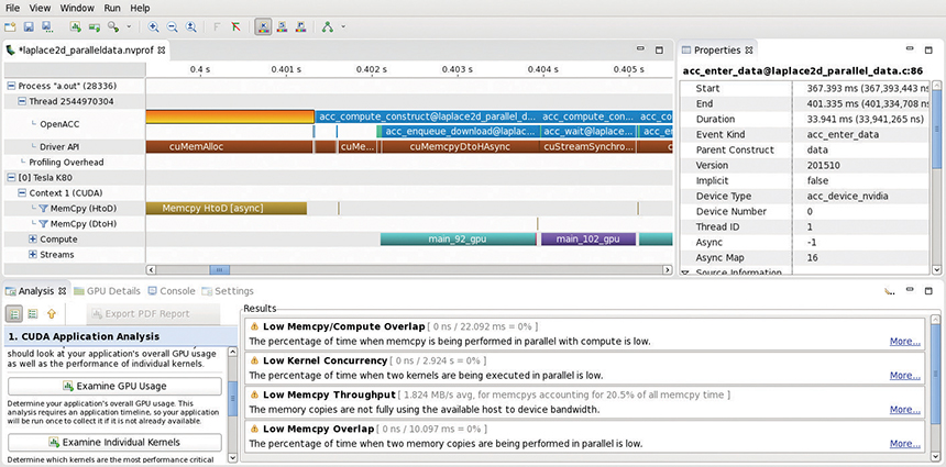
Because the GUI (nvvp) is not always available, nvprof can export the analysis results in a file to be imported by nvvp, or it can directly print text output to stdout or a specified file. Listing 3.2 shows an example analysis for a C program with OpenACC directives, which solves the 2D Laplace equation with the Jacobi iterative method.17 It shows the most runtime-consuming GPU tasks (kernels and memory copies), CUDA API calls, and OpenACC activities. Optimization efforts should focus on these hot spots. Note that nvprof is simply prepended to the executable program. When no options are used, the output for an OpenACC program with a CUDA target has three sections: global profile, CUDA API calls, and OpenACC activities. The list in each section is sorted by exclusive execution time.
17. https://devblogs.nvidia.com/parallelforall/getting-started-openacc/.
Figure 3.2 shows the nvvp visualization for the same example as mentioned earlier. The main display shows a timeline that visualizes the execution of OpenACC activities, CUDA driver API calls, and CUDA kernels that have been generated by the PGI 16.10 (community edition)18 compiler for a Tesla K80 GPU. The properties of the selected region are shown on the upper right of the figure. The region is an OpenACC enter data region with duration of about 33ms followed by a compute region. The respective CUDA API calls and CUDA kernels are shown in the underlying timeline bars. This illustrates the implementation of OpenACC constructs in the CUDA programming model in a timeline view. The nvvp profiler also provides summary profile tables, chart views, and a guided analysis (see the bottom half of Figure 3.2), information that supports programmers in identifying performance issues and optimization opportunities. You can use nvvp directly to analyze an application binary. It also allows loading a performance report that has been generated with nvprof or nvvp.
18. As of July 2017, PGI 17.4 is the most recent community edition; see https://www.pgroup.com/products/community.htm.
Listing 3.2 Exemplary nvprof usage and output for an iterative Jacobi solver
nvprof ./laplace2d_oacc
. . .
==50330== Profiling result:
Time(%) Time Calls Avg Min Max Name
58.25% 1.30766s 1000 1.3077ms 1.3022ms 1.3212ms main_92_gpu
40.12% 900.64ms 1000 900.64us 887.69us 915.98us main_102_gpu
0.55% 12.291ms 1000 12.290us 12.128us 12.640us main_92_gpu_red
0.54% 12.109ms 1004 12.060us 864ns 2.7994ms [CUDA memcpy HtoD]
. . .
==50330== API calls:
Time(%) Time Calls Avg Min Max Name
45.24% 1.31922s 1005 1.3127ms 9.2480us 1.3473ms cuMemcpyDtoHAsync
31.28% 912.13ms 3002 303.84us 2.7820us 2.4866ms cuStreamSynchroni
9.86% 287.63ms 1 287.63ms 287.63ms 287.63ms cuDeviceCtxRetain
9.55% 278.42ms 1 278.42ms 278.42ms 278.42ms cuDeviceCtxRelease
1.55% 45.202ms 3000 15.067us 12.214us 566.93us cuLaunchKernel
. . .
==50330== OpenACC (excl):
Time(%) Time Calls Avg Min Max Name
54.73% 1.32130s 1000 1.3213ms 1.2882ms 1.3498ms acc_enqueue_download@laplace2d_oacc.c:92
37.49% 905.04ms 1000 905.04us 347.17us 1.0006ms acc_wait@laplace2d_oacc.c:102
2.52% 60.780ms 1 60.780ms 60.780ms 60.780ms acc_enter_data@laplace2d_oacc.c:86
1.05% 25.246ms 1 25.246ms 25.246ms 25.246ms acc_exit_data@laplace2d_oacc.c:86
. . .
3.3.7 The Score-P Tools Infrastructure for Hybrid Applications
Score-P is an open source performance measurement infrastructure for several analysis tools, such as Vampir and CUBE (Cube Uniform Behavioral Encoding).19 Score-P has a large user community and supports programming models, such as MPI, OpenMP, SHMEM,20 CUDA, OpenCL, and OpenACC, as well as hardware counter and IO information.21 Score-P can generate profiles in the CUBE4 format and OTF222 traces.
19. Pavel Saviankou, Michael Knobloch, Anke Visser, and Bernd Mohr, “Cube v4: From Performance Report Explorer to Performance Analysis Tool,” Procedia Computer Science 51 (2015): 1343–1352.
20. http://www.openshmem.org/site/.
21. docs.cray.com/books/004-2178-002/06chap3.pdf.
22. Dominic Eschweiler et al., “Open Trace Format 2: The Next Generation of Scalable Trace Formats and Support Libraries,” Applications, Tools and Techniques on the Road to Exascale Computing 22 (2012): 481–490.
In comparison to the NVIDIA profiling tools, the focus is more on global optimizations of the program parallelization on all parallel layers. Hence, the Score-P tools scale to hundreds of thousands of processes, threads, and accelerator streams. The VI-HPS workshop material23 and the Score-P documentation24 provide detailed information on the Score-P analysis workflow, which can be summarized by the following steps.
23. http://www.vi-hps.org/training/material/.
24. https://silc.zih.tu-dresden.de/scorep-current/html/.
1. Prepare the measurement.
2. Generate a profile.
a. Visualize the profile with CUBE.
b. Estimate the trace file size.
c. Create a filtering file.
3. Generate a trace.
a. (Optionally) Automatically analyze trace file.
b. Visualize the trace with Vampir.
Before the measurement starts, the executable must be prepared. For OpenACC programs, the simplest way is to prepend scorep --cuda --openacc before the compiler command and recompile the application. The options cuda and openacc link the respective measurement components for CUDA and OpenACC into the binary. Typing scorep --help prints a summary of all available options.
The measurement itself is influenced by several environment variables. The variable scorep-info config-vars shows a list of all measurement configuration variables with a short description. Dedicated to OpenACC is the variable SCOREP_OPENACC_ENABLE, which accepts a comma-separated list of features.
• regions: Record OpenACC regions or directives.
• wait: Record OpenACC wait operations.
• enqueue: Record OpenACC enqueue kernel, upload, and download operations.
• device_alloc: Record OpenACC device memory deallocation or deallocation as a counter.
• kernel_properties: Record kernel name as well as the gang, worker, and vector size for kernel launch operations.
• variable_names: Record variable names for OpenACC data allocation and enqueue upload or download.
As defined in the OpenACC 2.5 specification, you must statically link the profiling library into the application, or you must specify the path to the shared library by setting ACC_PROFLIB=/path/to/shared/library or LD_PRELOAD=/path/to/shared/library. Score-P’s OpenACC profiling library is located in Score-P’s lib directory and is called libscorep_adapter_openacc_events.so.
To record additional information for CUDA targets, the environment variable SCOREP_CUDA_ENABLE can be specified. Relevant options are as follows.
• driver: Record the run time of calls to CUDA driver API.
• kernel: Record CUDA kernels.
• memcpy: Record CUDA memory copies.
• gpumemusage: Record CUDA memory allocations or deallocations as counter.
• flushatexit: Flush the CUDA activity buffer at program exit.
The amount of device memory to store device activities can be set with the environment variable SCOREP_CUDA_BUFFER (value in bytes), if needed.
You should carefully select the events to record to avoid unnecessary measurement overhead. For example, OpenACC enqueue operations are typically very short regions, and the CUDA driver feature includes similar information by tracking API functions such as cuLaunchKernel. There is an option to track the device memory allocations and deallocations in both the OpenACC and the CUDA features. A recommended low-overhead setup would use regions and wait from the OpenACC features, and kernel and memcpy from the CUDA features, an approach that supplies enough information to correlate OpenACC directives with CUDA device activities.
Figure 3.3 shows the profile visualization with the CUBE GUI for a hybrid MPI/OpenMP/OpenACC program (molecular dynamics code from Indiana University25). Selecting the exclusive runtime in the Metric tree box on the left of the figure, the CUDA kernel accel_296_gpu is dominating the runtime on the GPU (with 73.63 sec) as shown in the Flat view in the center. Immediately after the kernel launch, the host starts waiting for its completion (code location is int_ion_mix_acc.f in line 296). The System tree on the right shows the distribution of the execution time over processes, threads, and GPU streams.
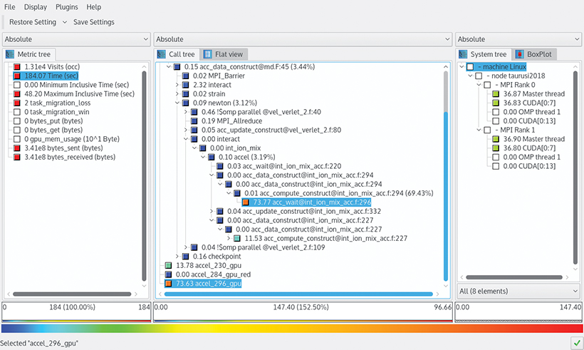
Note: Color coding (if you’re viewing this electronically) or shading (if you’re reading the paper version) highlights high values of a metric.
Figure 3.4 shows the Vampir visualization of an OTF2 trace that has been generated from the SPEC ACCEL26 363.swim benchmark. The selected time interval illustrates the level of detail that can be investigated using tracing. The timeline at the top of the figure shows a host stream (captioned Master thread) that triggers activities on the CUDA device stream (captioned CUDA[0:13]). Data transfers are visualized as black lines between two execution streams. Details on the selected data transfer are shown on the lower right in the Context View box. Each region in the timelines can be selected to get additional information. The Function Summary box on the upper right provides profile information of the selected time interval in the program execution. The runtime-dominating regions are an OpenACC launch in line 92 of file swim.f, and an OpenACC wait operation in line 124 of the same file. The CUDA stream shows some CUDA kernels (in orange if you’re viewing this electronically), but most of the time the GPU is idle. The lower timeline highlights regions on the critical path, which is the longest path in the program execution that does not contain any wait states. Optimizing regions that are not on the critical path has no effect on the total program run time.
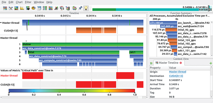
Note: The GUI provides several timeline views and statistical displays. All CUDA kernels are on the critical path (lower timeline), making them reasonable optimization targets.
26. Guido Juckeland et al., “SPEC ACCEL: A Standard Application Suite for Measuring Hardware Accelerator Performance,” 5th International Workshop on Performance Modeling, Benchmarking and Simulation of High Performance Computer Systems (2014): 46–67.
OTF2 traces can provide additional OpenACC runtime information that is not available in CUBE profiles. If the feature kernel_properties has been set, kernel launch parameters such as gang, worker, and vector size are added to the trace. The feature variable_names includes the name of variables for OpenACC data allocation and OpenACC data movement. Furthermore, implicit OpenACC operations are annotated. Vampir visualizes this information in the Context View box or by generating metrics from these attributes as counters in the Counter Data Timeline or Performance Radar box. All Vampir views can be opened using the chart menu or the icons that are shown on the bar at the top of Figure 3.4.
3.3.8 TAU Performance System
TAU is a versatile performance analysis tool suite that supports all parallel programming paradigms and parallel execution platforms. It enables performance measurement (profiling and tracing) of hybrid parallel applications and can capture the inner workings of OpenACC programs to identify performance problems for both host and device. The integrated TAU Performance System is open source and includes tools for source analysis (PDT), parallel profile analysis (ParaProf), profile data mining (PerfExplorer), and performance data management (TAUdb).
TAU provides both probe-based instrumentation and event-based sampling to observe parallel execution and generate performance data at the routine and statement levels. Although probe-based instrumentation relies on a pair of bracketed begin and end interval events, event-based sampling relies on generating a periodic interrupt when the program’s state is examined. Instrumentation in TAU is implemented by powerful mechanisms that expose code regions, such as routines and loops, at multiple levels: source, library, compiler, and binary. These features work consistently together and integrate with mechanisms to observe parallel performance events in runtime libraries. The latter include MPI, pthreads, OpenMP (via OMPT), CUDA (via CUPTI), and OpenACC.
The OpenACC 2.5 profiling interface is fully supported in TAU. Instrumentation-based performance measurement in TAU can use libraries such as PAPI to measure hardware performance counts, as well as Score-P, VampirTrace, and OTF2 to generate profiles and traces. In addition, TAU offers special measurement options that can capture performance of user-defined events, context events, calling parameters, execution phases, and so on.
TAU also supports event-based sampling (EBS) to capture performance data when the program’s execution is interrupted, either periodically by an interval timer or after a hardware counter overflow occurs. With sampling, fine-grained performance measurement at the statement level is possible, as is aggregation of all statement-level performance within a routine. TAU is one of very few systems that support both probe-based instrumentation and event-based sampling. It is the only tool that integrates the performance data at run time into a hybrid profile.27
27. Alan Morris, Allen D. Malony, Sameer Shende, and Kevin Huck, “Design and Implementation of a Hybrid Parallel Performance Measurement System,” Proc. International Conference on Parallel Processing (ICPP ’10) (2010).
To automatically activate a parallel performance measurement with TAU, the command tau_exec was developed. The command-line options to tau_exec determine the instrumentation functionality that is enabled. For example, to obtain a parallel performance profile for an MPI application that uses OpenACC, you can launch the application using this line:
% mpirun –-np <ranks> tau_exec -–openacc -ebs ./a.out
This command will collect performance data from the OpenACC profiling interface (-openacc) using instrumentation, as well as data from event-based sampling (-ebs). A separate profile will be generated for every MPI process in this case. Note that if OpenACC is offloaded to a CPU “device” that uses multithreading, every thread of execution will have its own profile.
TAU’s parallel profile browser, ParaProf, analyzes the profile generated when the application is launched by tau_exec. Figure 3.5 shows a view of ParaProf’s thread statistics window that gives the breakdown of performance data for the Cactus BenchADM benchmark28 from the PGI tutorial on OpenACC. Because event-based sampling was enabled for this performance experiment, ParaProf presents a hybrid performance view, where [SAMPLE] highlights an EBS sample measurement and [SUMMARY] shows the total contribution of events from that routine; “[CONTEXT]” highlights the “context” for EBS sample aggregation of the parent node. All other identifiers are instrumentation-based measurements.
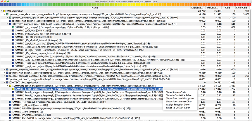
Figure 3.5 Exemplary TAU ParaProf thread statistics window showing the time spent in OpenACC and host code segments in a tree display
28. PGI, “Building Cactus BenchADM with PGI Accelerator Compilers,” PGI Insider, 2017, http://www.pgroup.com/lit/articles/insider/v1n2a4.htm.
In Figure 3.5, you see low-level routines that are called by the openacc_enter_data event for the bench_staggeredleapfrog2 routine (in green on electronic versions), which can be found in the StaggeredLeapfrog2_acc2.F file. Note that the routine calls the openacc_enqueue_upload event at line 369 in this file (just below the enter data event). This operation takes 5.725 seconds, as shown in the columns for exclusive and inclusive time. You also see samples generated in a routine __c_mcopy8 (also in green), a low-level routine from libpgc.so that presumably copies data. This routine executes for 6.03 seconds, as reported by the EBS measurement.29
29. Note that TAU can generate call-path profiles showing the nesting of events up to a certain call-path depth. A pair of environment variables is used to enable call-path profiling (TAU_CALLPATH) and to set the depth (TAU_CALLPATH_DEPTH). In this example, these variables were set to 1 and 1000, respectively.
The color coding (or shading, if you’re reading the paper edition) indicates performance intensity. For instance, the bench_staggeredleapfrog2_ routine at sample line 344 takes as much as 17.817 seconds of the total inclusive time of 35.853 seconds for the top level (identified as the TAU Application routine). As you see in Figure 3.5, by right-clicking and selecting a line of code, you can select the Show Source Code option to launch the source browser. The result is shown in Figure 3.6. It appears that this is a highly intensive computational loop that can be moved to the GPU using OpenACC constructs. You could easily turn on additional measurement, such as hardware counters, to investigate the performance behavior further.
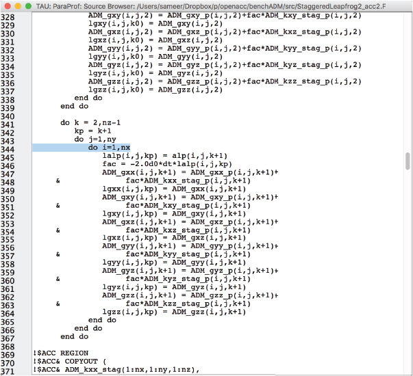
Figure 3.6 Exemplary TAU ParaProf source browser window showing the innermost loop on line 344, where the application spends 17.817 seconds
3.4 Identifying Bugs in OpenACC Programs
Program bugs typically cause unexpected or incorrect results, or errors that occur during the run time of the program. In general, a bug is a mistake made in the logic of a solution to a problem or in programming of that solution. Debugging is the process of finding and fixing a bug. It is a major part in the application development process and requires tools to help expose the bugs. Because OpenACC programs are executed on host and device, debugging is complicated. Additionally, the compiler has some leeway in interpreting several OpenACC directives, which might lead to “false bugs.”
The OpenACC specification does not define a debugging interface up to version 2.5. However, individual OpenACC compilers and runtimes provide environment variables to enable debugging output. You should consider this option before starting with tedious printf debugging, because the source code does not need to be changed. The GNU OpenACC runtime prints debug output if you set GOMP_DEBUG=1. The PGI compiler enables debug output with ACC_NOTIFY=1. Unfortunately, such debugging output can become lengthy, or the relevant information is not provided.
Thus, the following steps should help you systematically identify bugs in OpenACC programs.
1. Compile and execute the program without interpreting the OpenACC directives (without the -acc flag) to ensure that the bug arises in the context of the OpenACC implementation.
2. Use additional compiler output on OpenACC directives (e.g., -Minfo=accel) with the PGI compiler. This action typically provides information on the parallelization of loops and the implementation of data copy operations. Check whether the compiler does what it is supposed to do.
3. Check which version of the OpenACC specification is used by the compiler. Review the respective specification in uncertain cases.
4. Isolate the bug by, for example, moving code from OpenACC compute regions back to the host.
5. Use debuggers such as TotalView30 and Allinea DDT,31 which can be used for debugging at runtime in both host and device code.
30. http://www.roguewave.com/products-services/totalview.
31. https://www.allinea.com/products/ddt.
Parallel debuggers, such as DDT and TotalView, allow debugging of host and device code. This includes viewing variables and intrinsic values such as the threadIdx in CUDA kernels. Similarly, it is possible to set breakpoints in host and device code. Debugging of the device code is restricted to CUDA targets in the current version of both debuggers. Figure 3.7 shows exemplary debugging output of DDT for a CUDA program with a memory access error.32 Here, CUDA thread 254 tries to access an “illegal lane address” and causes a signal to occur. At this point, the respective pointer can be investigated, and the issue can be traced.
32. https://www.allinea.com/blog/debugging-cuda-dynamic-parallelism.
![Screenshot of a program stopped window overlapping the window Allinea DDT v4-0-BRANCH[Trial Version].](http://images-20200215.ebookreading.net/13/3/3/9780134694306/9780134694306__openacc-for-programmers__9780134694306__graphics__03fig07.jpg)
Figure 3.7 Parallel debugging with Allinea DDT supporting OpenACC with CUDA target devices Image courtesy of Allinea.
3.5 Summary
Several tools are available to help developers analyze their OpenACC code to get correct and high-performing OpenACC applications. Programming tools for OpenACC must cope with the concept of computation offloading, and this means that performance analysis and debugging must be performed on the host and the accelerator.
OpenACC 2.5 provides a profiling interface to gather events from an OpenACC runtime. Information on the accelerator performance must be acquired based on the target APIs used for the respective accelerator. Tools such as Score-P and TAU measure those performance data on both the host and the accelerator. Furthermore, they let you investigate programs that additionally use interprocess communication and multithreading.
Because the OpenACC compiler generates the device code, you would think you would not need to debug OpenACC compute kernels. But it is still possible to have logic and coding errors. Also, there are several other sources of errors that can be detected based on compiler or runtime debugging output. Tools such as TotalView and DDT support the debugging of OpenACC programs on host and CUDA devices.
Debugging and performance analysis are not one-time events. Because the compiler has some leeway in implementing the specification and because there are many different accelerators, optimizations can differ for each combination of compiler and accelerator. The same thing applies to bugs, which may occur only for a specific combination of compiler and accelerator. Software tools simplify the process of debugging and performance analysis. Because OpenACC is about performance, profile-driven program development is recommended. With the available tools, you can avoid do-it-yourself solutions.
3.6 Exercises
For a better understanding of compiling, analyzing, and debugging of OpenACC programs, we accelerate the Game of Life (GoL) with OpenACC. The C code appears in Listing 3.3.
The Game of Life is a cellular automaton that has been developed by mathematician John Horton Conway. The system is based on an infinite two-dimensional orthogonal grid. Each cell has eight neighbors and can have one of two possible states: dead or alive. Based on an initial pattern, further generations are determined with the following rules.
• Any dead cell with exactly three living neighbors becomes a living cell.
• Any living cell with two or three living neighbors lives on to the next generation.
• Any living cell with more than three or fewer than two living neighbors dies.
The program uses a two-dimensional stencil that sums up the eight closest neighbors and applies the game rules. The initial state can be randomly generated. Ghost cells are used to implement periodic boundary conditions. Cells are not updated until the end of the iteration.
Listing 3.3 Game of Life: CPU code
#include <stdio.h>
#include <stdlib.h>
void gol(int *grid, int *newGrid, cons tint dim) {
int i,j;
// copy ghost rows
for (i = 1; i <= dim; i++) {
grid[(dim+2)*(dim+1)+i] = grid[(dim+2)+i];
grid[i] = grid[(dim+2)*dim + i];
}
// copy ghost columns
for (i = 0; i <= dim+1; i++) {
grid[i*(dim+2)+dim+1] = grid[i*(dim+2)+1];
grid[i*(dim+2)] = grid[i*(dim+2) + dim];
}
// iterate over the grid
for (i = 1; i <= dim; i++) {
for (j = 1; j <= dim; j++) {
int id = i*(dim+2) + j;
int numNeighbors =
grid[id+(dim+2)] + grid[id-(dim+2)] // lower + upper
+ grid[id+1] + grid[id-1] // right + left
+ grid[id+(dim+3)] + grid[id-(dim+3)] // diagonal right
+ grid[id-(dim+1)] + grid[id+(dim+1)];// diagonal left
// the game rules (0=dead, 1=alive)
if (grid[id] == 1 && numNeighbors < 2)
newGrid[id] = 0;
else if (grid[id] == 1
&& (numNeighbors == 2 || numNeighbors == 3))
newGrid[id] = 1;
else if (grid[id] == 1 && numNeighbors > 3)
newGrid[id] = 0;
else if (grid[id] == 0 && numNeighbors == 3)
newGrid[id] = 1;
else
newGrid[id] = grid[id];
}
}
// copy new grid over, as pointers cannot be switched on the
// device (the CPU code could switch pointers only)
for (i = 1; i <= dim; i++) {
for (j = 1; j <= dim; j++) {
int id = i*(dim+2) + j;
grid[id] = newGrid[id];
}
}
}
int main(int argc, char* argv[])
{
int i, j, it, total;
// grid dimension (without ghost cells)
int dim = 1024;
if (argc > 1) dim = atoi(argv[1]);
// number of game steps
int itEnd = 1 << 11;
if (argc > 2) itEnd = atoi(argv[2]);
// grid array with dimension dim + ghost columns and rows
int arraySize = (dim+2) * (dim+2);
// current grid
int *grid = (int*)malloc(arraySize * sizeof(int)); // result grid
int *newGrid = (int*) malloc(arraySize * sizeof(int));
// assign initial population randomly
srand(1985); // pseudo random with a fixed seed
for(i = 1; i <= dim; i++) {
for(j = 1; j <= dim; j++) {
int id = i*(dim+2) + j;
grid[id] = rand() % 2;
}
}
for (it = 0; it < itEnd; it++){
gol( grid, newGrid, dim );
}
// sum up alive cells
total = 0; // total number of alive cells
for (i = 1; i <= dim; i++) {
for (j = 1; j <= dim; j++) {
int id = i*(dim+2) + j;
total += grid[id];
}
}
printf("Total Alive: %d
", total);
return 0;
}
The following tasks demonstrate the tools presented in this chapter. Use a profile-driven approach to accelerate GoL with OpenACC.
1. Measure the runtime of the sequential CPU code that implements the game of life per Listing 3.3. Use 1024 as grid dimension and 2048 steps. What is dominating the runtime of the CPU code? The runtime can be easily measured by prepending time before the executable.
2. Add OpenACC compute directives to execute one game step (iteration) on the device.
a. Compile the code using, for example, pgcc –acc gol_acc.c –o gol_acc.
b. Use –Minfo=accel with the PGI compiler to spot potential issues.
c. If necessary, use ACC_NOTIFY=1 to identify when an error occurs or alternatively (and if available), use DDT or TotalView to find bugs.
d. Make sure that the grid and newGrid arrays are available on the device. Add a respective clause to the compute construct, if necessary.
e. Identify loops without dependencies between iterations, and add respective loop constructs (#pragma acc loop independent).
f. Measure the runtime of the OpenACC program.
3. Use nvprof to profile the program. What is dominating the device runtime or is preventing the device from computing?
4. Use the data construct (or data enter or exit constructs) to avoid unnecessary host-device data movement between game iterations. Verify the result using nvprof or nvvp.
5. Count all living cells in parallel on the device using the OpenACC parallel construct.
6. Use Score-P to analyze the final OpenACC program.
a. Instrument the program using Score-P.
b. Set all required environment variables to capture OpenACC events and eventually CUDA or OpenCL device activity.
c. Generate a profile, and visualize it with the CUBE GUI.
d. What is dominating the runtime on the host? Which kernels are dominating the device runtime?
e. Measure the effect of gang, worker, and vector clauses on loop constructs. Try different values. The performance might depend on the grid size.
i. Add kernel_properties to SCOREP_OPENACC_ENABLE.
ii. Generate a trace file and visualize it with Vampir.
iii. Select the OpenACC kernel launch regions to get details on the launch properties.
iv. Which OpenACC runtime operations have been implicitly generated?