
Chapter 10. Advanced OpenACC
Jeff Larkin, NVIDIA
With the basics of OpenACC programming well in hand, this chapter discusses two advanced OpenACC features for maximizing application performance. The first feature is asynchronous operations, which allow multiple things to happen at the same time to better utilize the available system resources, such as a GPU, a CPU, and the PCIe connection in between. The second feature is support for multiple accelerator devices. The chapter discusses two ways that an application can utilize two or more accelerator devices to increase performance: one using purely OpenACC, and the other combining OpenACC with the Message Passing Interface (MPI).
10.1 Asynchronous Operations
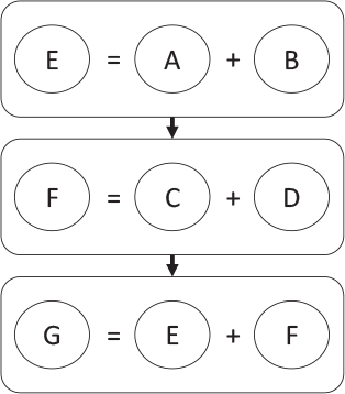
Programming is often taught by developing a series of steps that, when completed, achieve a specific result. If I add E = A + B and then F = C + D, then I can add G = E + F and get the sum of A, B, C, and D, as shown in Figure 10.1.
Our brains often like to think in an ordered list of steps, and that influences the way we write our programs, but in fact we’re used to carrying out multiple tasks at the same time. Take, for instance, cooking a spaghetti dinner. It would be silly to cook the pasta, and then the sauce, and finally the loaf of bread. Instead, you will probably let the sauce simmer while you bake the bread and, when the bread is almost finished, boil the pasta so that all the parts of the meal will be ready when they are needed. By thinking about when you need each part of the meal and cooking the parts so that they all complete only when they are needed, you can cook the meal in less time than if you’d prepared each part in a separate complete step. You also would better utilize the kitchen by taking advantage of the fact that you can have two pots and the oven working simultaneously.
By thinking of your operations as a series of dependencies, rather than a series of steps, you open yourself to running the steps in potentially more efficient orders, possibly even in parallel. This is a different sort of parallelism than we have discussed so far in this book. The chapters before this one focus on data parallelism, or performing the same action on many different data locations in parallel. In the case of the spaghetti dinner analogy, we’re discussing task-based parallelism, or exposing different tasks, each of which may or may not be data parallel, that can be executed concurrently.
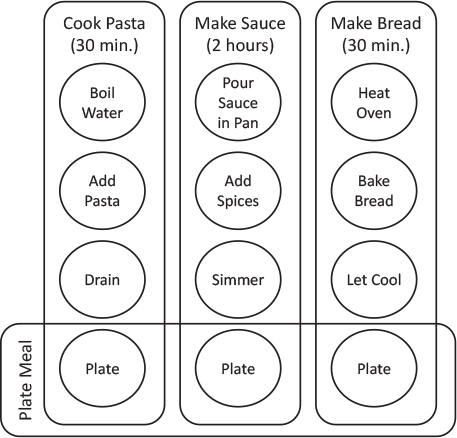
Let us look at the spaghetti dinner example a little more closely. You can treat cooking the pasta, preparing the sauce, and baking the bread as three separate operations in cooking the dinner. Cooking the pasta takes roughly 30 minutes, because it involves bringing the water to a boil, actually cooking the pasta, and then draining it when it is done. Making the sauce takes quite a bit longer, roughly two hours from putting the sauce in a pot, adding seasoning, and then simmering so that the seasoning takes effect. Baking the bread is another 30-minute operation, involving heating the oven, baking the bread, and then allowing the bread to cool. Finally, when these operations are complete, you can plate and eat your dinner.
If I did each of these operations in order (in any order), then the entire process would take three hours, and at least some part of my meal would be cold. To understand the dependencies between the steps, let’s look at the process in reverse.
1. To plate the meal, the pasta, sauce, and bread must all be complete.
2. For the pasta to be complete, it must have been drained, which requires that it has been cooked, which requires that the water has been brought to a boil.
3. For the sauce to be ready, it must have simmered, which requires that the seasoning has been added, and the sauce has been put into a pot.
4. For the bread to be done, it must have cooled, before which it must have been baked, which requires that the oven has been heated.
From this, you can see that the three parts of the meal do not need to be prepared in any particular order, but each has its own steps that do have a required order. To put it in parallel programming terms, each step within the larger tasks has a dependency on the preceding step, but the three major tasks are independent of each other. Figure 10.2 illustrates this point. The circles indicate the steps in cooking the dinner, and the rounded rectangles indicate the steps that have dependencies. Notice that when each task reaches the plating step, it becomes dependent on the completion of the other tasks. Therefore, where the rounded rectangles overlap is where the cook needs to synchronize the tasks, because the results of all three tasks are required before you can move on; but where the boxes do not cross, the tasks can operate asynchronously from each other.
Asynchronous programming is a practice of exposing the dependencies in the code to enable multiple independent operations to be run concurrently across the available system resources. Exposing dependencies does not guarantee that independent operations will be run concurrently, but it does enable this possibility. In the example, what if your stove has only one burner? Could you still overlap the cooking of the pasta with the simmering of the sauce? No, because both require the same resource: the burner. In this case, you will need to serialize those two tasks so that one uses the burner as soon as the other is complete, but the order in which those tasks complete is still irrelevant. Asynchronous programming is also the practice of removing synchronization between independent steps, and hence the term asynchronous. It takes great care to ensure that necessary synchronization is placed in the code to produce consistently correct results, but when done correctly this style of programming can better utilize available resources.
10.1.1 Asynchronous OpenACC Programming
By default, all OpenACC directives are synchronous with the host thread, meaning that after the host thread has sent the required data and instructions to the accelerator, the host thread will wait for the accelerator to complete its work before continuing execution. By remaining synchronous with the host thread OpenACC ensures that operations occur in the same order when run on the accelerator as when run in the original program, thereby ensuring that the program will run correctly with or without an accelerator.
This is rarely the most efficient way to run the code, however, because system resources go unused while the host is waiting for the accelerator to complete. For instance, on a system having one CPU and one GPU, which are connected via PCIe, then at any given time either the CPU is computing, the GPU is computing, or the PCIe bus is copying data, but no two of those resources are ever used concurrently. If we were to expose the dependencies in our code and then launch our operations asynchronously from the host thread, then the host thread would be free to send more data and instructions to the device or even participate in the calculation. OpenACC uses the async clause and wait directive to achieve exactly this.
Asynchronous Work Queues
OpenACC uses asynchronous work queues to expose dependencies between operations. Anything placed into the same work queue will be executed in the order it was enqueued. This is a typical first-in, first-out (FIFO) queue. Operations placed in different work queues can execute in any order, no matter which was enqueued first. When the results of a particular queue (or all queues) are needed, the programmer must wait (or synchronize) on the work queue (or queues). Referring to Figure 10.2, the rounded rectangles could each represent a separate work queue, and the steps should be put into that queue in the order in which they must be completed.
OpenACC identifies asynchronous queues with non-negative integer numbers, so all work enqueued to queue 1, for instance, will complete in order and operate independently of work enqueued in queue 2. The specification also defines several special work queues. If acc_async_sync is specified as the queue, then all directives placed into the queue will become synchronous with the host thread, something that is useful for debugging. If the queue acc_async_noval is used, then the operation will be placed into the default asynchronous queue.
The async Clause
Specific directives are placed into work queues by adding the async clause to the directive. This clause may be added to parallel and kernels regions and the update directive. This clause optionally accepts a non-negative integer value or one of the special values previously discussed. If no parameter is given to the async clause, then it will behave as if the acc_async_noval queue was specified, often referred to as the default queue. Listing 10.1 demonstrates the use of the async clause in C/C++, both with and without the optional parameter.
Listing 10.1 Example of async clause in C/C++
// The next directive updates the value of A on the device
// asynchronously of the host thread and in queue #1.
#pragma acc update device(A[:N]) async(1)
// The next directive updates the value of B on the device
// and may execute before the previous update has completed.
// This update has been placed in the default queue.
#pragma acc update device(B[:N]) async
// The host thread will continue execution, even before the
// above updates have.
The wait Directive
Once work has been made asynchronous, it’s necessary to later synchronize when the results of that work are needed. Failure to synchronize will likely produce incorrect results. This can be achieved in OpenACC by using either the wait directive or the wait clause. The wait directive identifies a place in the code that the encountering thread cannot pass until all asynchronous work up to that point in the program has completed. The directive optionally accepts a work queue number so that the program waits only for the work in the specified work queue to complete, and not all asynchronous work. Listing 10.2 demonstrates the use of the wait directive in C/C++.
Listing 10.2 Example of wait directive in C/C++
// The next directive updates the value of A on the device
// asynchronously of the host thread and in queue #1.
#pragma acc update device(A[:N]) async(1)
// The host thread will continue execution, even before the
// above updates have completed.
// The next directive updates the value of B on the device
// and may execute before the previous update has completed.
// This update has been placed in queue #2.
#pragma acc update device(B[:N]) async(2)
// The next directive updates the value of C on the device
// and may execute before the previous update has completed.
// This update has been placed in the default queue.
#pragma acc update device(C[:N]) async
// When the program encounters the following directive, it will
// block further execution until the data transfer in queue #1
// has completed.
#pragma acc wait(1)
// When the program encounters the following directive, it will
// wait for all remaining asynchronous work from this thread to
// complete before continuing.
#pragma acc wait
Perhaps rather than insert a whole new directive into the code to force this synchronization, you would rather force an already existing directive to wait on a particular queue. This can be achieved with the wait clause, which is available on many directives. Listing 10.3 demonstrates this in both C and C++.
Listing 10.3 Example of wait directive in C/C++
// The next directive updates the value of A on the device
// asynchronously of the host thread and in queue #1.
#pragma acc update device(A(:N)) async(1)
// The next directive updates the value of B on the device
// and may execute before the previous update has completed.
// This update has been placed in queue #2.
#pragma acc update device(B[:N]) async(2)
// The host thread will continue execution, even before the
// above updates have completed.
// The next directive creates a parallel loop region, which it
// enqueues in work queue #1, but waits on queue #2. Queue 1
// will wait here until all prior work in queue #2 has completed
// and then continue executing.
#pragma acc parallel loop async(1) wait(2)
for (int i=0 ; i < N; i++) {
C[i] = A[i] + B[i]
}
// When the program encounters the following directive, it will
// wait for all remaining asynchronous work from this thread
// into any queue to complete before continuing.
#pragma acc wait
Joining Work Queues
When placing work into multiple work queues, eventually you need to wait for work to complete in both queues before execution moves forward. The most obvious way to handle such a situation is to insert a wait directive for each queue and then move forward with the calculation. Although this technique works for ensuring correctness, it results in the host CPU blocking execution until both queues have completed and could create bubbles in one or both queues while no work is available to execute, particularly if one queue requires more time to execute than the other. Instead of using the host CPU to synchronize the queues, it’s possible to join the queues together at the point where they need to synchronize by using an asynchronous wait directive. The idea of asynchronously waiting may seem counterintuitive, so consider Listing 10.4. The code performs a simple vector summation but has separate loops for initializing the A array, initializing the B array, and finally summing them both into the C array. Note that this is a highly inefficient way to perform a vector sum, but it is written only to demonstrate the concept discussed in this section. The OpenACC directives place the work of initializing A and B into queues 1 and 2, respectively. The summation loop should not be run until both queues 1 and 2 have completed, so an asynchronous wait directive is used to force queue 1 to wait until the work in queue 2 has completed before moving forward.
On first reading, the asynchronous wait directive may feel backward, so let’s break down what it is saying. First, the directive says to wait on queue 2, but then it also says to place this directive asynchronously into work queue 1 so that the host CPU is free to move on to enqueue the summation loop into queue 1 and then wait for it to complete. Effectively, queues 1 and 2 are joined together at the asynchronous wait directive and then queue 1 continues with the summation loop. By writing the code in this way you enable the OpenACC runtime to resolve the dependency between queues 1 and 2 on the device, for devices that support this, rather than block the host CPU. This results in better utilization of system resources, because the host CPU no longer must idly wait for both queues to complete.
Listing 10.4 Example of asynchronous wait directive in C/C++
#pragma acc data create(A[:N],B[:N],C[:N])
{
#pragma acc parallel loop async(1)
for(int i=0; i<N; i++)
{
A[i] = 1.f;
}
#pragma acc parallel loop async(2)
for(int i=0; i<N; i++)
{
B[i] = 2.f;
}
#pragma acc wait(2) async(1)
#pragma acc parallel loop async(1)
for(int i=0; i<N; i++)
{
C[i] = A[i] + B[i];
}
#pragma acc update self(C[0:N]) async(1)
// Host CPU free to do other, unrelated work
#pragma acc wait(1)
}
Interoperating with CUDA Streams
When developing for an NVIDIA GPU, you may need to mix OpenACC’s asynchronous work queues with CUDA streams to ensure that any dependencies between OpenACC and CUDA kernels or accelerated libraries are properly exposed. Chapter 9 demonstrates that it is possible to use the acc_get_cuda_stream function to obtain the CUDA stream associated with an OpenACC work queue. For instance, in Listing 10.5, you see that acc_get_cuda_stream is used to obtain a CUDA stream, which is then used by the NVIDIA cuBLAS library to allow the arrays populated in queue 1 in OpenACC to then safely be passed between the asynchronous loop in line 6, the asynchronous library call in line 15, and the update directive in line 16. By getting the CUDA stream associated with queue 1 in this way, you can still operate asynchronously from the host thread while ensuring that the dependency between the OpenACC directives and the cublas function is met. This feature is useful when you are adding asynchronous CUDA or library calls to a primarily OpenACC application.
Listing 10.5 Example of acc_get_cuda_stream function
1 cudaStream_t stream = (cudaStream_t)acc_get_cuda_stream(1);
2 status = cublasSetStream(handle,stream);
3
4 #pragma acc data create(a[:N],b[:N])
5 {
6 #pragma acc parallel loop async(1)
7 for(int i=0;i<N;i++)
8 {
9 a[i] = 1.f;
10 b[i] = 0.f;
11 }
12
13 #pragma acc host_data use_device(a,b)
14 {
15 status = cublasSaxpy(handle, N, &alpha, a, 1, b, 1);
16 #pragma acc update self(b[:N]) async (1)
17 #pragma acc wait(1)
18 }
It is also possible to work in reverse, associating a CUDA stream used in an application with a particular OpenACC work queue. You achieve this by calling the acc_set_cuda_stream function with the CUDA stream you wish to use and the queue number with which it should be associated. In Listing 10.6, you see that I have reversed my function calls so that I first query which stream the cublas library will use and then associate that stream with OpenACC’s work queue 1. Such an approach may be useful when you are adding OpenACC to a code that already has extensive use of CUDA or accelerated libraries, because you can reuse existing CUDA streams.
Listing 10.6 Example of acc_set_cuda_stream function
1 status = cublasSetStream(handle,stream);
2 acc_set_cuda_stream(1, (void*)stream);
3
4 #pragma acc data create(a[:N],b[:N])
5 {
6 #pragma acc parallel loop async(1)
7 for(int i=0;i<N;i++)
8 {
9 a[i] = 1.f;
10 b[i] = 0.f;
11 }
12
13 #pragma acc host_data use_device(a,b)
14 {
15 status = cublasSaxpy(handle, N, &alpha, a, 1, b, 1);
16 }
17 #pragma acc update self(b[:N]) async (1)
18 #pragma acc wait(1)
19 }
These examples strictly work on NVIDIA GPUs with CUDA, but OpenACC compilers using OpenCL have a similar API for interoperating with OpenCL work queues.
10.1.2 Software Pipelining
This section demonstrates one technique that is enabled by asynchronous programming: software pipelining. Pipelining is not the only way to take advantage of asynchronous work queues, but it does demonstrate how work queues can allow better utilization of system resources by ensuring that multiple operations can happen at the same time. For this example, we will use a simple image-filtering program that reads an image, performs some manipulations on the pixels, and then writes the results back out. Listing 10.7 shows the main filter routine, which has already been accelerated with OpenACC directives.
Listing 10.7 Baseline OpenACC image-filtering code
const int filtersize = 5;
const double filter[5][5] =
{
0, 0, 1, 0, 0,
0, 2, 2, 2, 0,
1, 2, 3, 2, 1,
0, 2, 2, 2, 0,
0, 0, 1, 0, 0
};
// The denominator for scale should be the sum
// of non-zero elements in the filter.
const float scale = 1.0 / 23.0;
void blur5(unsigned restrict char *imgData,
unsigned restrict char *out, long w, long h, long ch, long step)
{
long x, y;
#pragma acc parallel loop collapse(2) gang vector
copyin(imgData[0:w * h * ch])
copyout(out[0:w * h * ch])
for ( y = 0; y < h; y++ )
{
for ( x = 0; x < w; x++ )
{
float blue = 0.0, green = 0.0, red = 0.0;
for ( int fy = 0; fy < filtersize; fy++ )
{
long iy = y - (filtersize/2) + fy;
for ( int fx = 0; fx < filtersize; fx++ )
{
long ix = x - (filtersize/2) + fx;
if ( (iy<0) || (ix<0) ||
(iy>=h) || (ix>=w) ) continue;
blue += filter[fy][fx] *
(float)imgData[iy * step + ix * ch];
green += filter[fy][fx] *
(float)imgData[iy * step + ix * ch + 1];
red += filter[fy][fx] *
(float)imgData[iy * step + ix * ch + 2];
}
}
out[y * step + x * ch] = 255 - (scale * blue);
out[y * step + x * ch + 1 ] = 255 - (scale * green);
out[y * step + x * ch + 2 ] = 255 - (scale * red);
}
}
}
We start by analyzing the current application performance using the PGI compiler, an NVIDIA GPU, and the PGProf profiling tool. Figure 10.3 shows a screen shot of PGProf, which shows the GPU timeline for the filter application. For reference, the data presented is for a Tesla P100 accelerator and an 8,000×4,051 pixel image. Notice that copying the image data to and from the device takes nearly as much time as actually performing the filtering of the image. The program requires 8.8ms to copy the image to the device, 8.2ms copying the data from the device, and 20.5ms performing the filtering operation.
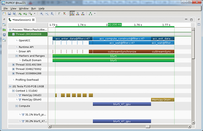
The most significant performance limiter in this application is the time spent copying data between the CPU and the GPU over PCIe. Unfortunately, you cannot remove that time, because you do need to perform those copies for the program to work, so you need to look for ways to overlap the data copies with the GPU work. If you could completely overlap both directions of data transfers with the filtering kernel, then the total run time would drop to only 20.5ms, which is a speedup of 1.8×, so this is the maximum speedup you can obtain by optimizing to hide the data movement.
How can you overlap the data transfers, though, if you need to get the data to the device before you start and cannot remove it until you have computed the results? The trick is to recognize that you do not need all of the data on the device to proceed; you need only enough to kick things off. If you could break the work into discrete parts, just as you did with cooking dinner earlier, then you can operate on each smaller part independently and potentially overlap steps that do not require the same system resource at the same time. Image manipulation is a perfect case study for this sort of optimization, because each pixel of an image is independent of all the others, so the image itself can be broken into smaller parts that can be independently filtered.
Blocking the Computation
Before we can pipeline the operations, we need to refactor the code to operate on chunks, commonly referred to as blocks, of independent work. The code, as it is written, essentially has one block. By adding a loop around this operation and adjusting the bounds of the existing loops to avoid redundant work, you can make the code do exactly the same thing it does currently, but in two or more blocks. You write the code to break the operation only along rows, because this means that each block is contiguous in memory, something that will be important in later steps. It should also be written to allow for any number of blocks from one up to the height of the image, giving you maximum flexibility later to find just the right number of blocks. Listing 10.8 shows the new code with the addition of the blocking loop.
Listing 10.8 Blocked OpenACC image-filtering code
1 void blur5_blocked(unsigned restrict char *imgData,
2 unsigned restrict char *out,
3 long w, long h, long ch, long step)
4 {
5 long x, y;
6 const int nblocks = 8;
7
8 long blocksize = h/ nblocks;
9 #pragma acc data copyin(imgData[:w*h*ch],filter)
10 copyout(out[:w*h*ch])
11 for ( long blocky = 0; blocky < nblocks; blocky++)
12 {
13 // For data copies we include the ghost zones for filter
14 long starty = blocky * blocksize;
15 long endy = starty + blocksize;
16 #pragma acc parallel loop collapse(2) gang vector
17 for ( y = starty; y < endy; y++ )
18 {
19 for ( x = 0; x < w; x++ )
20 {
21 float blue = 0.0, green = 0.0, red = 0.0;
22 for ( int fy = 0; fy < filtersize; fy++ )
23 {
24 long iy = y - (filtersize/2) + fy;
25 for ( int fx = 0; fx < filtersize; fx++ )
26 {
27 long ix = x - (filtersize/2) + fx;
28 if ( (iy<0) || (ix<0) ||
29 (iy>=h) || (ix>=w) ) continue;
30 blue += filter[fy][fx] *
31 (float)imgData[iy * step + ix * ch];
32 green += filter[fy][fx] * (float)imgData[iy * step + ix *
33 ch + 1];
34 red += filter[fy][fx] * (float)imgData[iy * step + ix *
35 ch + 2];
36 }
37 }
38 out[y * step + x * ch] = 255 - (scale * blue);
39 out[y * step + x * ch + 1 ] = 255 - (scale * green);
40 out[y * step + x * ch + 2 ] = 255 - (scale * red);
41 }
42 }
43 }
44 }
There are a few important things to note from this code example. First, we have blocked only the computation, and not the data transfers. This is because we want to ensure that we obtain correct results by making only small changes to the code with each step. Second, notice that within each block we calculate the starting and ending rows of the block and adjust the y loop accordingly (lines 11–13). Failing to make this adjustment would produce correct results but would increase the run time proportionally to the number of blocks. With this change in place, you will see later in Figure 10.4 that the performance is slightly worse than the original. This is because we have introduced a little more overhead to the operation to manage the multiple blocks of work. However, this additional overhead will be more than compensated for in the final code.
Blocking the Data Movement
Now that the computation has been blocked and is producing correct results, it’s time to break up the data movement between the host and the accelerator to place it within blocks as well. To do this, you first need to change the data clauses for the imgData and out arrays to remove the data copies around the blocking loop (see Listing 10.9, line 9). This can be done by changing both arrays to use the create data clause. Next, you add two acc update directives: one at the beginning of the block’s execution (line 17) to copy the input data from imgData before the computation, and another after the computation to copy the results back into the out array (line 48).
Our image filter has one subtlety that needs to be addressed during this step. The filter operation for element [i][j] of the image requires the values from several surrounding pixels, particularly two to left and right, and two up and down. This means that for the filter to produce the same results, when you copy a block’s portion of imgData to the accelerator you also need to copy the two rows before that block and the two after, if they exist. These additional rows are frequently referred to as a halo or ghost zone, because they surround the core part of the data. In Listing 10.9, notice that, to accommodate the surrounding rows, the starting and ending rows for the update directive are slightly different from the starting and ending rows of the compute loops. Not all computations require this overlapping, but because of the nature of the image filter, this application does. The full code for this step is found in Listing 10.9.
Listing 10.9 Blocked OpenACC image-filtering code with separate update directives
1 void blur5_update(unsigned restrict char *imgData,
2 unsigned restrict char *out, long w, long h,
3 long ch, long step)
4 {
5 long x, y;
6 const int nblocks = 8;
7
8 long blocksize = h/ nblocks;
9 #pragma acc data create(imgData[w*h*ch],out[w*h*ch])
10 copyin(filter)
11 {
12 for ( long blocky = 0; blocky < nblocks; blocky++)
13 {
14 // For data copies we include ghost zones for the filter
15 long starty = MAX(0,blocky * blocksize - filtersize/2);
16 long endy = MIN(h,starty + blocksize + filtersize/2);
17 #pragma acc update
18 device(imgData[starty*step:(endy-starty)*step])
19 starty = blocky * blocksize;
20 endy = starty + blocksize;
21 #pragma acc parallel loop collapse(2) gang vector
22 for ( y = starty; y < endy; y++ )
23 {
24 for ( x = 0; x < w; x++ )
25 {
26 float blue = 0.0, green = 0.0, red = 0.0;
27 for ( int fy = 0; fy < filtersize; fy++ )
28 {
29 long iy = y - (filtersize/2) + fy;
30 for ( int fx = 0; fx < filtersize; fx++ )
31 {
32 long ix = x - (filtersize/2) + fx;
33 if ( (iy<0) || (ix<0) ||
34 (iy>=h) || (ix>=w) ) continue;
35 blue += filter[fy][fx] *
36 (float)imgData[iy * step + ix * ch];
37 green += filter[fy][fx] *
38 (float)imgData[iy * step + ix * ch + 1];
39 red += filter[fy][fx] *
40 (float)imgData[iy * step + ix * ch + 2];
41 }
42 }
43 out[y * step + x * ch] = 255 - (scale * blue);
44 out[y * step + x * ch + 1 ] = 255 - (scale * green);
45 out[y * step + x * ch + 2 ] = 255 - (scale * red);
46 }
47 }
48 #pragma acc update self(out[starty*step:blocksize*step])
49 }
50 }
51 }
Again, you need to run the code and check the results before moving to the next step. You see in Figure 10.4 that the code is again slightly slower than the previous version because of increased overhead, but that will soon go away.
Making It Asynchronous
The last step in implementing software pipelining using OpenACC is to make the whole operation asynchronous. Again, the key requirement for making an operation work effectively asynchronously is to expose the dependencies or data flow in the code so that independent operations can be run concurrently with sufficient resources. You will use OpenACC’s work queues to expose the flow of data through each block of the image. For each block, the code must update the device, apply the filter, and then update the host, and it must be done in that order. This means that for each block these three operations should be put in the same work queue. These operations for different blocks may be placed in different queues, so the block number is a convenient way to refer to the work queues. There is overhead involved in creating new work queues, so it is frequently a best practice to reuse some smaller number of queues throughout the computation.
Because we know that we are hoping to overlap a host-to-device copy, accelerator computation, and a device-to-host copy, it seems as if three work queues should be enough. For each block of the operation you use the block number, modulo 3 to signify which queue to use for a given block’s work. As a personal preference, I generally choose to reserve queue 0 for special situations, so for this example we will always add 1 to the queue number to avoid using queue 0.
Listing 10.10 shows the code from this step, which adds the async clause to both update directives and the parallel loop, using the formula just discussed to determine the work queue number. However, one critical and easy-to-miss step remains before we can run the code: adding synchronization to the end of the computation. If we did not synchronize before writing the image to a file, we’d almost certainly produce an image that’s only partially filtered. The wait directive in line 52 of Listing 10.10 prevents the host thread from moving forward until after all asynchronous work on the accelerator has completed. The final code for this step appears in Listing 10.10.
Listing 10.10 Final, pipelined OpenACC filtering code with asynchronous directives
1 void blur5_pipelined(unsigned restrict char *imgData,
2 unsigned restrict char *out, long w, long h,
3 long ch, long step)
4 {
5 long x, y;
6 const int nblocks = 8;
7
8 long blocksize = h/ nblocks;
9 #pragma acc data create(imgData[w*h*ch],out[w*h*ch])
10 {
11 for ( long blocky = 0; blocky < nblocks; blocky++)
12 {
13 // For data copies we include ghost zones for the filter
14 long starty = MAX(0,blocky * blocksize - filtersize/2);
15 long endy = MIN(h,starty + blocksize + filtersize/2);
16 #pragma acc update
17 device(imgData[starty*step:(endy-starty)*step])
18 async(blocky%3+1)
19 starty = blocky * blocksize;
20 endy = starty + blocksize;
21 #pragma acc parallel loop collapse(2) gang vector
22 async(blocky%3+1)
23 for ( y = starty; y < endy; y++ )
24 {
25 for ( x = 0; x < w; x++ )
26 {
27 float blue = 0.0, green = 0.0, red = 0.0;
28 for ( int fy = 0; fy < filtersize; fy++ )
29 {
30 long iy = y - (filtersize/2) + fy;
31 for ( int fx = 0; fx < filtersize; fx++ )
32 {
33 long ix = x - (filtersize/2) + fx;
34 if ( (iy<0) || (ix<0) ||
35 (iy>=h) || (ix>=w) ) continue;
36 blue += filter[fy][fx] *
37 (float)imgData[iy * step + ix * ch];
38 green += filter[fy][fx] *
39 (float)imgData[iy * step + ix * ch + 1];
40 red += filter[fy][fx] *
41 (float)imgData[iy * step + ix * ch + 2];
42 }
43 }
44 out[y * step + x * ch] = 255 - (scale * blue);
45 out[y * step + x * ch + 1 ] = 255 - (scale * green);
46 out[y * step + x * ch + 2 ] = 255 - (scale * red);
47 }
48 }
49 #pragma acc update self(out[starty*step:blocksize*step])
50 async(blocky%3+1)
51 }
52 #pragma acc wait
53 }
54 }
What is the net result of these changes? First, notice in Table 10.1 that the run time of the whole operation has now improved by quite a bit. Compared with the original version, you see an improvement of 1.8×, which is roughly what we predicted earlier for fully overlapped code. Figure 10.5 is another timeline from the PGProf, which shows that we have achieved exactly what we set out to do. Notice that nearly all of the data movement is overlapped with computation on the GPU, making it essentially free. The little bit of data transfer at the beginning and end of the computation is offset by a small amount of overlap between subsequent filter kernels as each kernel begins to run out of work and the next one begins to run. You can experiment with the number of blocks and find the optimal value, which may vary depending on the machine on which you are running. In Figure 10.5, we are obviously operating on eight blocks.
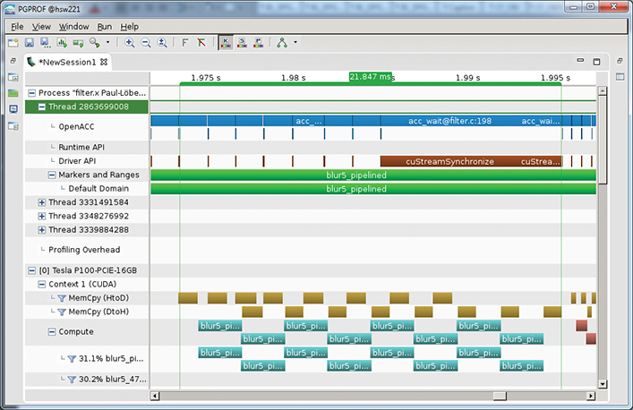
Table 10.1 PGProf timeline for baseline image filter
OPTIMIZATION STEP |
TIME (MS) |
SPEEDUP |
Baseline |
43.102 |
1.00× |
Blocked |
45.217 |
0.95× |
Blocked with update |
52.161 |
0.83× |
Asynchronous |
23.602 |
1.83× |
10.2 Multidevice Programming
Many systems are now built with not only one, but several accelerator devices. This section discusses ways to extend existing code to divide work across multiple devices.
10.2.1 Multidevice Pipeline
In the preceding section, you modified an image-filtering program to operate over blocks of the image so that you could overlap the cost of transferring the requisite data to and from the device with computation on the device. Here is something to consider about that example: If each block is fully independent of the other blocks and manages its data correctly, do those blocks need to be run on the same device? The answer, of course, is no, but how do you send blocks to different devices using OpenACC?
To do that, OpenACC provides the acc_set_device_num function. This function accepts two arguments: a device type and a device number. With those two pieces of information, you should be able to choose any device in your machine and direct your work to that device. Once you have called acc_set_device_num, all OpenACC directives encountered by the host thread up until the next call to acc_set_device_num will be handled by the specified device. Each device will have its own copies of the data (if your program is running on a device that has a distinct memory) and its own work queues. Also, each host thread can set its own device number, something you’ll take advantage of in this section.
The OpenACC runtime library provides routines for querying and setting both the device type (e.g., NVIDIA GPU, AMD GPU, Intel Xeon Phi, etc.) and the device number. With these API routines you can direct both your data and compute kernels to different devices as needed. Let us first look at the routines for querying and setting the device type.
Listing 10.11 demonstrates the usage of acc_get_device_type and acc_set_device_type to query and set the type of accelerator to use by default. Setting only the type means that the OpenACC runtime will still choose the specific device within that type to use. You can take even more control and specify the exact device number within a device type to use.
Listing 10.11 Example usage of setting and getting OpenACC device type
1 #include <stdio.h>
2 #include <openacc.h>
3 int main()
4 {
5 int error = 0;
6 acc_device_t myDev = -1;
7
8 acc_set_device_type(acc_device_nvidia);
9 myDev = acc_get_device_type();
10 if ( myDev != acc_device_nvidia )
11 {
12 fprintf(stderr, "Wrong device type returned! %d != %d
",
13 (int)myDev, (int)acc_device_nvidia);
14 error = -1;
15 }
16 return error;
17 }
Listing 10.12 demonstrates the acc_set_device_num and acc_get_device_num routines. These listings also demonstrate the acc_get_num_devices routine, which is used to learn how many devices of a particular type are available. This information can be useful in ensuring that the application is portable to any machine, no matter how many accelerators are installed.
Listing 10.12 Example usage of getting the number of devices, setting the current device, and getting the current device number
1 #include <stdio.h>
2 #include <openacc.h>
3 int main()
4 {
5 int numDevices = -1, myNum = -1;
6 numDevices = acc_get_num_devices(acc_device_nvidia);
7 acc_set_device_num(acc_device_nvidia,0);
8 myNum = acc_get_device_num(acc_device_nvidia);
9
10 printf("Using device %d of %d.
", myNum, numDevices);
11
12 return 0;
13 }
Let’s extend the pipelined example from the preceding section to send the chunks of work to all available devices. Although I am running on an NVIDIA Tesla P100, I don’t want to assume that other users will have a machine that matches my own, so I will specify acc_device_default as my device type. This is a special device type value that tells the compiler that I don’t care what specific device type it chooses. On my testing machine, I could also have used acc_device_nvidia, because that best describes the accelerators in my machine. I have chosen to use OpenMP to assign a CPU thread to each of my accelerator devices. This is not strictly necessary—a single thread could send work to all devices—but in my opinion this simplifies the code because I can call acc_set_device once in each thread and not worry about it again.
Listing 10.13 Multidevice image-filtering code using OpenACC and OpenMP
1 #include <openacc.h>
2 #include <omp.h>
3 void blur5_pipelined_multi(unsigned restrict char *imgData,
4 unsigned restrict char *out,
5 long w, long h, long ch, long step)
6 {
7 int nblocks = 32;
8
9 long blocksize = h/ nblocks;
10 #pragma omp parallel
11 num_threads(acc_get_num_devices(acc_device_default))
12 {
13 int myid = omp_get_thread_num();
14 acc_set_device_num(myid,acc_device_default);
15 int queue = 1;
16 #pragma acc data create(imgData[w*h*ch],out[w*h*ch])
17 {
18 #pragma omp for schedule(static)
19 for ( long blocky = 0; blocky < nblocks; blocky++)
20 {
21 // For data copies we include ghost zones for the filter
22 long starty = MAX(0,blocky * blocksize - filtersize/2);
23 long endy = MIN(h,starty + blocksize + filtersize/2);
24 #pragma acc update device
25 (imgData[starty*step:(endy-starty)*step])
26 async(queue)
27 starty = blocky * blocksize;
28 endy = starty + blocksize;
29 #pragma acc parallel loop collapse(2) gang vector async(queue)
30 for ( long y = starty; y < endy; y++ )
31 {
32 for ( long x = 0; x < w; x++ )
33 {
34 float blue = 0.0, green = 0.0, red = 0.0;
35 for ( int fy = 0; fy < filtersize; fy++ )
36 {
37 long iy = y - (filtersize/2) + fy;
38 for ( int fx = 0; fx < filtersize; fx++ )
39 {
40 long ix = x - (filtersize/2) + fx;
41 if ( (iy<0) || (ix<0) ||
42 (iy>=h) || (ix>=w) ) continue;
43 blue += filter[fy][fx] *
44 (float)imgData[iy * step + ix * ch];
45 green += filter[fy][fx] *
46 (float)imgData[iy * step + ix * ch + 1];
47 red += filter[fy][fx] *
48 (float)imgData[iy * step + ix * ch + 2];
49 }
50 }
51 out[y * step + x * ch] = 255 - (scale * blue);
52 out[y * step + x * ch + 1 ] = 255 - (scale * green);
53 out[y * step + x * ch + 2 ] = 255 - (scale * red);
54 }
55 }
56 #pragma acc update self(out[starty*step:blocksize*step])
57 async(queue)
58 queue = (queue%3)+1;
59 }
60 #pragma acc wait
61 }
62 }
63 }
In line 10 of Listing 10.13, you start by querying the number of available devices and then use that number to spawn an OpenMP parallel region with that number of threads. In line 14, which is run redundantly by all threads in the OpenMP region, you set the device number that will be used by each individual thread, using the thread number to select the device. Notice also that you change from using a simple modulo operator to set the work queue number to having a per-thread counter. This change prevents the modulo from assigning all chunks from a given device to a reduced number of queues when certain device counts are used. The remainder of the code is unchanged, because each device will have its own data region (line 16) and will have its own work queues.
Table 10.2 shows the results of running the code on one, two, and four GPUs (three is skipped because it would not divide the work evenly). Notice that you see a performance improvement with each additional device, but it is not a strict doubling as the number of devices doubles. It is typical to see some performance degradation as more devices are added because of additional overhead brought into the calculation by each device.
Table 10.2 Multiple-device pipeline timings
NUMBER OF DEVICES |
TIME (MS) |
SPEEDUP |
1 |
20.628 |
1.00× |
2 |
12.041 |
1.71× |
4 |
7.769 |
2.66× |
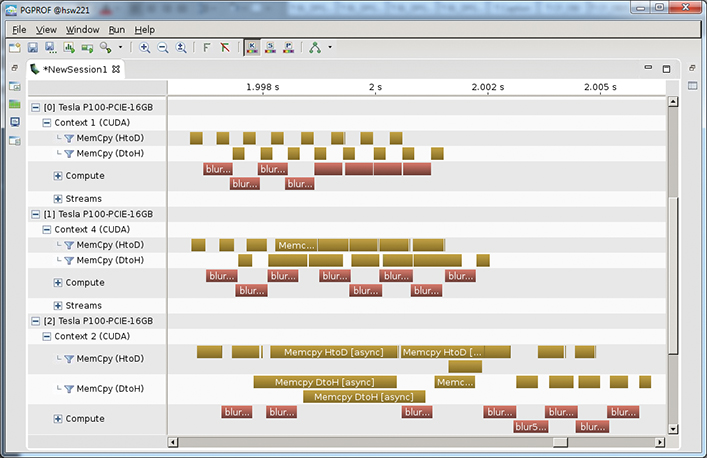
Figure 10.4, presented earlier, shows another screenshot from PGProf, in which you can clearly see overlapping data movement and computation across multiple devices. Note that in the example code it was necessary to run the operation twice so that the first time would absorb the start-up cost of the multiple devices and the second would provide fair timing. In short-running benchmarks like this one, such a step is needed to prevent the start-up time from dominating the performance. In real, long-running applications, this is not necessary because the start-up cost will be hidden by the long runtime.
10.2.2 OpenACC and MPI
Another common method for managing multiple devices with OpenACC is to use MPI to divide the work among multiple processes, each of which is assigned to work with an individual accelerator. MPI is commonly used in scientific and high-performance computing applications, so many applications already use MPI to divide work among multiple processes.
This approach has several advantages and disadvantages compared with the approach used in the preceding section. For one thing, application developers are forced to consider how to divide the problem domain into discrete chunks, which are assigned to different processors, thereby effectively isolating each GPU from the others to avoid possible race conditions on the same data. Also, because the domain is divided among multiple processes, it is possible that these processes may span multiple nodes in a cluster, and this increases both the available memory and the number of accelerators available. For applications already using MPI to run in parallel, using MPI to manage multiple accelerators often requires fewer code changes compared with managing multiple devices using OpenACC alone. Using existing MPI also has the advantage that non-accelerated parts of the code can still use MPI parallelism to avoid a serialization slowdown due to Amdahl’s law. When you’re dealing with GPUs and other discrete accelerators, it is common for a system to have more CPU cores than it does discrete accelerators. In these situations, it is common to either share a single accelerator among multiple MPI ranks or to thread within each MPI rank to better utilize all system resources.
When you are using MPI to utilize multiple discrete accelerators, to obtain the best possible performance it is often necessary to understand how the accelerators and host CPUs are connected. For instance, if a system has two multicore CPU sockets and four GPU cards, as shown in Figure 10.6, then it’s likely that each CPU socket will be directly connected to two GPUs but will have to communicate with the other two GPUs by way of the other CPU, and this reduces the available bandwidth and increases the latency between the CPU and the GPU.
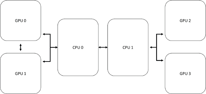
Furthermore, in some GPU configurations each pair of GPUs may be able to communicate directly with each other, but only indirectly with GPUs on the opposite socket. Best performance is achieved when each rank is assigned to the nearest accelerator, something known as good accelerator affinity. Although some MPI job launchers will handle assigning a GPU to each MPI rank, you should not count on this behavior; instead you should use the acc_set_device_num function to manually assign a particular accelerator to each MPI rank. By understanding how MPI assigns ranks to CPU cores and how the CPUs and accelerators are configured, you can assign the accelerator affinity so that each rank is communicating with the nearest available accelerator, thereby maximizing host-device bandwidth and minimizing latency. For instance, in Figure 10.6, you would want to assign GPU0 and GPU1 to ranks physically assigned to CPU0 and GPU2, and assign GPU3 to ranks physically assigned to CPU1. This is true whether or not ranks are assigned to the CPUs in a round-robin manner, packed to CPU0 and then CPU1, or in some other order.
Many MPI libraries can now communicate directly with accelerator memory, particularly on clusters utilizing NVIDIA GPUs, which support a feature known as GPUDirect RDMA (remote direct memory access). When you are using one of these MPI libraries it’s possible to use the host_data directive to pass accelerator memory to the library, as shown in Chapter 9 and discussed next.
MPI Without Direct Memory Access
Let’s first consider an OpenACC application using MPI that cannot use an accelerator-aware MPI library. In this case, any call to an MPI routine would require the addition of an update directive before, after, or potentially before and after the library call, depending on how the data are used. Although MPI does support asynchronous sending and receiving of messages, the MPI API does not understand OpenACC’s concept of work queues, and therefore either update directives must be synchronous or a wait directive must appear before any MPI function that sends data. Similarly, an OpenACC update directive should not appear directly following an asynchronous MPI function that receives data, but only after synchronous communication or the associated MPI_Wait call; in this way, you ensure that the data in the host buffer are correct before they are updated to the device. Listing 10.14 shows several common communication patterns for interacting between OpenACC and an MPI library that is not accelerator aware.
Listing 10.14 Common patterns for MPI communication with OpenACC updates
// When using MPI_Sendrecv or any blocking collective, it is
// necessary to have an update before and after.
#pragma acc update self(u_new[offset_first_row:m-2])
MPI_Sendrecv(u_new+offset_first_row, m-2, MPI_DOUBLE, t_nb, 0,
u_new+offset_bottom_boundary, m-2,
MPI_DOUBLE, b_nb, 0,
MPI_COMM_WORLD, MPI_STATUS_IGNORE);
#pragma acc update device(u_new[offset_bottom_boundary:m-2])
// When using either MPI_Send or MPI_Isend, an update is
// required before the MPI call
#pragma acc update self(u_new[offset_first_row:m-2])
MPI_Send(u_new+offset_first_row, m-2, MPI_DOUBLE, t_nb, 0, i
MPI_COMM_WORLD);
// When using a blocking receive, an update may appear
// immediately after the MPI call.
MPI_Recv(u_new+offset_bottom_boundary, m-2, MPI_DOUBLE, b_nb, 0,
MPI_COMM_WORLD, MPI_STATUS_IGNORE);
#pragma acc update device(u_new[offset_bottom_boundary:m-2])
// When using a nonblocking receives, it is necessary to MPI_Wait
// before using an OpenACC update
MPI_Irecv(u_new+offset_bottom_boundary, m-2, MPI_DOUBLE, b_nb, 0,
MPI_COMM_WORLD, MPI_STATUS_IGNORE, &request);
MPI_Wait(&request, MPI_STATUS_IGNORE);
#pragma acc update device(u_new[offset_bottom_boundary:m-2])
The biggest drawback to this approach is that all interactions between OpenACC and MPI require a copy through host memory. This means that there can never be effective overlapping between MPI and OpenACC and that it may be necessary to communicate the data over the PCIe bus twice as often. If possible, this approach to using MPI with OpenACC should be avoided.
MPI with Direct Memory Access
Having an MPI implementation that is accelerator aware greatly simplifies the mixture of OpenACC and MPI. It is no longer necessary to manually stage data through the host memory using the update directive, but rather the MPI library can directly read from and write to accelerator memory, potentially reducing the bandwidth cost associated with the data transfer and simplifying the code. Just because an MPI library is accelerator aware does not necessarily guarantee that data will be sent directly between the accelerator memories. The library may still choose to stage the data through host memory or perform a variety of optimizations invisibly to the developer. This means that it is the responsibility of the library developer, rather than the application developer, to determine the best way to send the message on a given machine. As discussed in Chapter 9, the OpenACC host_data directive is used for passing device pointers to host libraries. This same directive can be used to pass accelerator memory to an accelerator-aware MPI library. Note, however, that if the same code is used with a non-accelerator-aware library a program crash will occur. Listing 10.15 demonstrates some common patterns for using host_data to pass device arrays into the MPI library. This method has far fewer caveats to highlight than the preceding one.
Listing 10.15 Example using OpenACC host_data directive with accelerator-enabled MPI
// By using an accelerator-aware MPI library, host_data may be
// used to pass device memory directly into the library.
#pragma acc host_data use_device(u_new)
{
MPI_Sendrecv(u_new+offset_first_row, m-2, MPI_DOUBLE, t_nb, 0,
u_new+offset_bottom_boundary, m-2,
MPI_DOUBLE, b_nb, 0,
MPI_COMM_WORLD, MPI_STATUS_IGNORE);
}
// Because the Irecv is writing directly to accelerator memory
// only the MPI_Wait is required to ensure the data are current,
// no additional update is required.
#pragma acc host_data use_device(u_new)
{
MPI_Irecv(u_new+offset_bottom_boundary, m-2, MPI_DOUBLE, b_nb, 0,
MPI_COMM_WORLD, MPI_STATUS_IGNORE, &request);
}
MPI_Wait(&request, MPI_STATUS_IGNORE );
One advantage of this approach over the other one comes when you’re using asynchronous MPI calls. In the earlier case the update of the device data could not occur until after MPI_Wait has completed, because the update may copy stale data to the device. Because the MPI library is interacting with accelerator memory directly, MPI_Wait will guarantee that data have been placed in the accelerator buffer, removing the overhead of updating the device after the receive has completed. Additionally, the MPI library can invisibly perform optimizations of the way the messages are transferred, such as pipelining smaller message blocks, a feature that may be more efficient than directly copying the memory or manually staging buffers through host memory, for all the same reasons pipelining was beneficial in the earlier example.
This section has presented two methods for utilizing multiple accelerator devices with OpenACC. The first method uses OpenACC’s built-in acc_set_device_num function call to direct data and work to specific devices. In particular, OpenMP threads are used to assign a different host thread to each device, although this is not strictly necessary. The second method uses MPI to partition work across multiple processes, each of which utilizes a different accelerator. This approach is often simpler to implement in scientific code, because such code frequently uses MPI partitioning, meaning that non-accelerated code may still run across multiple MPI ranks. Both approaches can take advantage of multiple accelerators in the same node, but only the MPI approach can be used to manage multiple accelerators on different nodes. Which approach will work best depends on the specific needs of the application, and both techniques can be used together in the same application.
The source code in GitHub accompanying this chapter (check the Preface for a link to GitHub) includes the image filter pipeline code used in this chapter and a simple OpenACC + MPI application that can be used as examples.
10.3 Summary
You can exploit advanced techniques using OpenACC asynchronous execution and management of multiple devices. These techniques are designed to maximize application performance by improving the way the application uses all available resources. Asynchronous execution decouples work on the host from work on the accelerator, including data transfers between the two, allowing the application to use the host, accelerator, and any connecting bus concurrently, but only if all data dependencies are properly handled. Multidevice support extends this idea by allowing a program to utilize all available accelerators for maximum performance.
10.4 Exercises
1. The source code for the image-filtering example used in this chapter has been provided at the GitHub site shown in the Preface. You should attempt to build and understand this sample application.
2. You should experiment to determine the best block size for your machine. Does changing the image size affect the result? Does changing the accelerator type change the result?