
Chapter 3: Formatting Output
Writing a Blank Line between Each Row
Using the FORMAT= Column Modifier to Format Output
Concatenating Character Strings
Inserting Text and Constants between Columns
Using Scalar Expressions with Selected Columns
Grouping Data with Summary Functions
Subsetting Groups with the HAVING Clause
Formatting Output with the Output Delivery System
Sending Output to a SAS Data Set
Converting Output to Rich Text Format
Exporting Data and Output to Excel
Programmers want and expect to be able to format output in a variety of ways. The SQL procedure has forged innovative ways to enhance the appearance of output including double-spacing rows of output, concatenating two or more columns, inserting text and constants between selected columns, displaying column headers for derived fields, and much more. As a value-added feature, the SQL procedure (not part of ANSI-standard SQL—see the “Introduction” section of this book) can be integrated with the Output Delivery System to enhance and format output in ways not otherwise available. As you review the many examples in this chapter, the following points should be kept in mind:
As a language, PROC SQL consists of a standard set of statements and options to create, retrieve, alter, transform, and transfer data regardless of the operating system or where the data is located. These features provide tremendous power as well as control when integrating information from a variety of sources in a number of ways. Because emphasis is placed on PROC SQL’s data manipulation capabilities and not on its format and output capabilities, many programmers are unfamiliar with the SQL procedure’s output-producing side. Consequently, programmers resort to using report writers or special outputting tools to create the best looking output. To illustrate the virtues of PROC SQL in SAS, this chapter presents numerous examples of how output can be formatted and produced.
The ability to display a blank line between each row of output is available as a procedure option in PROC SQL. As with the PRINT procedure, specifying DOUBLE in the SQL procedure inserts a blank line between each physical row of output (NODOUBLE is the default). Setting this option is especially useful when one or more flowed lines spans or wraps in the output because it provides visual separation between each row of data. This example illustrates using the DOUBLE option to double-space output.
SQL Code
PROC SQL DOUBLE;
SELECT *
FROM INVOICE;
QUIT;
Results

To revert back to single-spaced output, the RESET statement can be specified as long as the QUIT statement has not been issued to turn off the SQL procedure. When PROC SQL is active, the RESET statement can be specified with or without options to reestablish each option’s original settings. All SQL options are reset to their original settings when RESET is specified without any options. When the RESET statement is specified with one or more options, only those options are reset. This example illustrates using the NODOUBLE option to turn off double-spaced output and reset printing to the default single-spaced output.
SQL Code
PROC SQL;
RESET NODOUBLE;
QUIT;
You can specify an SQL procedure option called NUMBER to display row numbers on output under the column heading Row. As with the Obs column produced by the PRINT procedure, the NUMBER option displays row numbers on output. The next example shows the NUMBER option being specified with the SQL procedure to display row numbers on output.
SQL Code
PROC SQL NUMBER;
SELECT PRODNUM,
UNITS,
UNITCOST
FROM PURCHASES;
QUIT;
Results


The SQL procedure supports the specification of a FORMAT= column modifier for purposes of providing instructions on how to write character and numeric data values by a query expression. The general syntax for writing a format follows:
<$>format<w>.<d>
where
$ is used to reference a character format and its absence references a numeric format.
format is the name of the desired SAS format or user-defined format to be used (see the SAS Language Reference: Dictionary, Fourth Edition for a complete listing and description of the available character, numeric, and date formats).
w references the format width, which is typically represented by the number of output columns used for the data.
d represents the optional decimal positioning for numeric data.
Referring to the example first shown in Chapter 2, “Working with Data in PROC SQL,” the next example illustrates the computation of a discounted value (80% of PRODCOST) from the PRODUCTS table, the assignment of a column alias of “Discount_Price” with the AS keyword, and the DOLLAR9.2 format applied to the resulting value with a FORMAT= column modifier.
SQL Code
PROC SQL;
SELECT PRODNAME,
PRODTYPE,
PRODCOST * 0.80 AS Discount_Price FORMAT=DOLLAR9.2
FROM PRODUCTS
ORDER BY 3;
QUIT;
Results

As was presented in Chapter 2, two or more strings can be concatenated to produce a combined and longer string of characters. The concatenation character string operator, which is represented by two vertical bars “||”, “!!”, or “¦¦” (depending on the operating system and keyboard being used), combines two or more strings or columns together to form a new string value. In the next example, the manufacturer city and manufacturer state columns from the MANUFACTURERS table are concatenated so that the second column immediately follows the first. Although the two character strings are successfully concatenated, the output illustrates potential problems as a result of using the concatenation operator.
The next example shows that because the first column has a “fixed” length, blanks are automatically padded to the entire length of the first concatenated column for each row of data. As a result of using the concatenation operator, the column headers for both columns are suppressed. Readers are cautioned that due to the loss of some or all of the column header information, a true understanding of the contents of the output may be in jeopardy.
SQL Code
PROC SQL;
SELECT manucity || manustat
FROM MANUFACTURERS;
QUIT;
Results

To make the preceding output appear a bit more readable and complete, you should consider a few modifications. First, column headers could be assigned as aliases with the AS operator. The maximum size of a user-defined column header is 32 bytes in length (adhering to SAS naming conventions). Finally, the TRIM function (which is described in Chapter 2, “Working with Data in PROC SQL”) could be used to remove trailing blanks from the city column. This allows the second column to act as a floating field.
SQL Code
PROC SQL;
SELECT TRIM(manucity) || manustat AS Headquarters
FROM MANUFACTURERS;
QUIT;
Results

Although the preceding output illustrates that some changes were made, it is still difficult to read. A few more cosmetic changes should be made to make it more aesthetically appealing and readable. In the next section, the output will be customized to give the data further separation.
At times, it is useful to be able to insert text and/or constants in query output. This enables special characters including symbols and comments to be inserted in the output. We can improve the output in the previous example by inserting a comma “,” and a single blank space between the manufacturer city and manufacturer state information. The final output illustrates an acceptable way to display columnar data using a “free-floating” presentation as opposed to fixed columns.
SQL Code
PROC SQL;
SELECT trim(manucity) || ‘, ‘ || manustat
As Headquarters
FROM MANUFACTURERS;
QUIT;
Results

Another method of automatically concatenating character strings, removing leading and trailing blanks, and inserting text and constants is with the CATX function. The next example shows the CATX function with a “, ” specified as a separator (a blank character immediately follows the comma) between character strings MANUCITY and MANUSTAT. Although a comma and blank character are successfully inserted between the MANUCITY and MANUSTAT columns, the output is automatically left justified conforming to the value assigned in the LINESIZE= system option.
SQL Code
PROC SQL;
SELECT CATX(‘, ’, manucity, manustat)
As Headquarters
FROM MANUFACTURERS;
QUIT;
Results

In computing terms, a scalar refers to a quantity represented by a single number or value. The value is not represented as an array or list of values, but as a single value. For example, the value 7 is a scalar value, but (0,0,7) is not. PROC SQL allows the use of scalar expressions and constants with selected columns. Typically, these expressions replace or augment one or more columns in the SELECT statement. To illustrate how a scalar expression is used, assume that a value of 7.5% representing the sales tax percentage is computed for each product in the PRODUCTS table. The results consist of the product name, product cost, and derived computed sales tax column.
Note: Although the computed column contains the results of the sales tax computation for each product, it does not contain a column heading.
SQL Code
PROC SQL;
SELECT prodname, prodcost,
.075 * prodcost
FROM PRODUCTS;
QUIT;
Results
In the next two examples, a column header or alias is assigned to the derived sales tax column computed in the previous example. Two methods exist for achieving this. As illustrated in the next example, the first method uses the AS keyword to assign a name to the derived column as well as to permit referencing the column later in the query.
SQL Code
PROC SQL;
SELECT prodname, prodcost,
.075 * prodcost AS Sales_Tax
FROM PRODUCTS;
QUIT;
Results

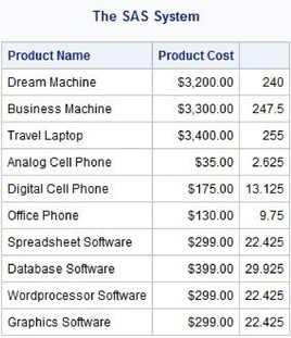
The next example illustrates the second method of assigning a column heading for the computed sales tax column with the LABEL= option. To further enhance the output’s readability, a numeric dollar format is specified.
Note: Because the next example is a query and the table is not being updated, the assigned attributes are only available for the duration of the step and are not permanently saved in the table’s record descriptor.
SQL Code
PROC SQL;
SELECT prodname, prodcost,
.075 * prodcost FORMAT=DOLLAR7.2
LABEL=’Sales Tax’
FROM PRODUCTS;
QUIT;
Results

By definition, tables are unordered sets of data. The data that comes from a table does not automatically appear in any particular order. To offset this behavior, the SQL procedure provides the ability to impose order in a table by using an ORDER BY clause. When used, this clause orders the query results according to the values in one or more selected columns; it must be specified after the FROM clause.
Rows of data can be ordered in ascending (default order) or descending (DESC) order for each column specified (ascending is the default order). To illustrate how selected columns of data can be ordered, let’s first view the PRODUCTS table and all its columns arranged in ascending order by product number (PRODNUM).
SQL Code
PROC SQL;
SELECT *
FROM PRODUCTS
ORDER BY prodnum;
QUIT;
Results

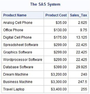
The next example uses the third column ordinal position in an ORDER BY clause to order and display the query results.
SQL Code
PROC SQL;
SELECT prodname, prodcost,
.075 * prodcost AS Sales_Tax
FROM PRODUCTS
ORDER BY 3;
QUIT;
Results
The next example illustrates a query that selects and orders multiple columns of data from the PRODUCTS table. Output is arranged first in ascending order by product type (PRODTYPE) and then within product type in descending order by product cost (PRODCOST). The code and output are shown.
SQL Code
PROC SQL;
SELECT prodname, prodtype, prodcost, prodnum
FROM PRODUCTS
ORDER BY prodtype, prodcost DESC;
QUIT;
Results

Occasionally it may be useful to display data in designated groups. A GROUP BY clause is used in these situations to aggregate and order groups of data using a designated column with the same value. When a GROUP BY clause is used without a summary function, SAS issues a warning in the SAS log with the message, “A GROUP BY clause has been transformed into an ORDER BY clause because neither the SELECT clause nor the optional HAVING clause of the associated table-expression referenced a summary function.” The GROUP BY clause is transformed into an ORDER BY clause and then processed.
When a GROUP BY clause is used without specifying a summary function in the SELECT statement, the entire table is treated as a single group and is ordered in ascending order. The next example illustrates a GROUP BY clause without any summary function specifications. Due to the absence of any summary functions, the GROUP BY clause is automatically transformed into an ORDER BY clause, with the rows being ordered in ascending order by product type (PRODTYPE).
SQL Code
PROC SQL;
SELECT prodtype,
prodcost
FROM PRODUCTS
GROUP BY prodtype;
QUIT;
Log Results
PROC SQL;
SELECT prodtype,
prodcost
FROM PRODUCTS
GROUP BY prodtype;
WARNING: A GROUP BY clause has been transformed into an ORDER BY clause because neither the SELECT clause nor the optional HAVING clause of the associated table-expression referenced a summary function.
QUIT;
Results

When a GROUP BY clause is used with a summary function, the rows are aggregated in a series of groups. This means that an aggregate function is evaluated on a group of rows and not on a single row at a time. Suppose that the least expensive product in each product type category (PRODTYPE) needs to be identified. A separate query for each product category could be specified using the MIN function to determine the cheapest product. But this would require separate runs to be executed—not a very good approach. A better way to do this would be to specify a GROUP BY clause in a single statement as follows.
SQL Code
PROC SQL;
SELECT prodtype,
MIN(prodcost) AS Cheapest
Format=dollar9.2 Label=’Least Expensive’
FROM PRODUCTS
GROUP BY prodtype;
QUIT;
Results

In the absence of an ORDER BY clause, the SQL procedure automatically sorts the results from a grouped query in the same order as specified in the GROUP BY clause. When both an ORDER BY clause and GROUP BY clause are specified for the same column(s) or column order, no additional processing occurs to satisfy the request. Because the ORDER BY clause and GROUP BY clause are not mutually exclusive, they can be used together. Internally, the GROUP BY clause first sorts the results on the grouping column(s) and then aggregates the rows of the query by the same grouping column.
But what happens when the column(s) specified in the ORDER BY clause and GROUP BY clause are not the same? In these situations, additional processing requirements are generally required. The additional processing, in a worse-case scenario, may require remerging summary statistics with the original data. In other cases, additional sorting requirements may be necessary. Suppose that information about the least expensive product in each product category is desired. But instead of automatically sorting the results in ascending order by product type, as before, the results will be displayed in ascending order by the least expensive product for each product type.
SQL Code
PROC SQL;
SELECT prodtype,
MIN(prodcost) AS Cheapest
Format=dollar9.2 Label=’Least Expensive’
FROM PRODUCTS
GROUP BY prodtype
ORDER BY cheapest;
QUIT;
Results

When processing groups of data, it is frequently useful to subset aggregated rows (or groups) of data. This way, aggregated data can be filtered one group at a time in contrast to filtering one row at a time. SQL provides a convenient way to subset (or filter) groups of data by using the GROUP BY clause and the HAVING clause. The HAVING clause is optional, but when specified is used in combination with the GROUP BY clause.
The HAVING clause is similar to the WHERE clause in that it specifies conditions that must be satisfied in order for results to become part of the subset. It differs from the WHERE clause in that it can refer to the results derived from summary functions after the aggregation of all observations for each of the groups. The groups that evaluate to true based on the HAVING clause are retained, and the groups that evaluate to false are automatically removed from consideration.
Suppose that you wanted to identify only those product groupings that have an average cost that is less than $400.00 from the PRODUCTS table. Your first inclination might be to use a summary function in a WHERE clause. But, this would not be valid because a WHERE clause restricts the number of rows selected. In contrast, the HAVING clause restricts the number of groups selected, and is always performed after the GROUP BY clause. For those already familiar with subqueries as discussed in Chapter 7, “Coding Complex Queries,” you could also approach the problem as a complex query. But, there is an easier and more straightforward way of identifying and selecting the desired product groups using the GROUP BY clause and HAVING clause, as follows.
SQL Code
PROC SQL;
SELECT prodtype,
AVG(prodcost)
FORMAT=DOLLAR9.2 LABEL=’Average Product Cost’
FROM PRODUCTS
GROUP BY prodtype
HAVING AVG(prodcost) <= 400.00;
QUIT;
Results

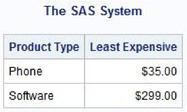
To illustrate the GROUP BY clause and the HAVING clause further, suppose you have a $400.00 spending limit and you want to identify the least expensive product within each product grouping from the PRODUCTS table. The next example returns only those product types that are within the $400.00 spending limit, as follows.
SQL Code
PROC SQL;
SELECT prodtype,
MIN(prodcost) AS Cheapest
FORMAT=DOLLAR9.2 LABEL=’Least Expensive’
FROM PRODUCTS
GROUP BY prodtype
HAVING Cheapest <= 400.00;
QUIT;
Results
When the WHERE clause, GROUP BY clause, and HAVING clause are used together in a SELECT statement, the WHERE clause is processed first. Then, the rows returned by the WHERE clause are grouped in accordance with the GROUP BY clause. Finally, the conditions specified in the HAVING clause are applied to the groups before the results are produced. The next example returns those software and hardware product types that are within the $400.00 spending limit.
SQL Code
PROC SQL;
SELECT prodtype,
AVG(prodcost) AS Average_Product_Cost
FORMAT=dollar12.2
FROM PRODUCTS
WHERE prodtype IN (‘Software’, ‘Hardware’)
GROUP BY prodtype
HAVING Average_Product_Cost < 400;
QUIT;
Results

SAS provides users with a familiar and automatic way to look at output in a listing file. Although easy to use, it is not extremely flexible when it comes to creating nice-looking output. The SAS Output Delivery System (ODS) provides many ways to format output by controlling the way it is accessed and formatted. Many output formats are available with ODS, including traditional SAS monospace font (i.e., Listing).
ODS was first introduced in version 7 as a way to improve the way traditional SAS output looks. It enables quality looking output to be produced without the need to import it into word processors such as Microsoft Word. Since then, many additional output formatting features and options are available for SAS users to take advantage of. With ODS, users have a powerful and easy way to create and access formatted procedure and DATA step output.
ODS statements are classified as global statements and are processed immediately by SAS. With built-in format engines, which are referred to as output destinations, ODS prepares output using special formats and layouts. Figure 3.1 illustrates the types of output that can be produced with ODS.
Figure 3.1: ODS Output Destinations
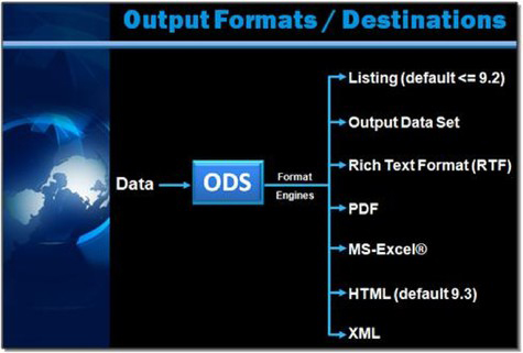
The PROC step and the DATA step produce output in the form of an output object to any and all open destinations. An output destination controls what format engine is turned on during a step or until another ODS statement is specified. One or more output destinations can be opened concurrently. When a destination is open, one or more output objects can be sent to it. Conversely, when a destination is closed, output objects are not sent to the destination.
Several really good ODS books are available for further study on this exciting facility including Output Delivery System: The Basics and Beyond, by Lauren Haworth, Cynthia L. Zender, and Michele Burlew; and Quick Results with the Output Delivery System, by Sunil Kumar Gupta.
Output produced by the SQL procedure can also be used as input to another vendor’s SQL, procedure, or DATA step. ODS provides an easy and consistent alternative for creating a SAS table of results. For users who are already familiar with ODS, this approach will consist of a simple process of specifying the OUTPUT destination in an ODS statement. For users who prefer a more traditional ANSI SQL approach, the CREATE TABLE statement (see Chapter 5, “Creating, Populating, and Deleting Tables,” for more details) will be the method of choice. Depending on the method you ultimately use, the advantage of creating a SAS table of output is a handy feature that all SAS users should become familiar with.
Although the CREATE TABLE statement is the standard method of creating a table in PROC SQL, the ODS OUTPUT statement can also be specified to produce a table. Using the ODS OUTPUT statement, the result table is a rectangular structure consisting of one or more rows and columns. In this example, the SQL procedure’s results are stored in object SQL_Results and are then sent to data set SQL_DATA using the ODS OUTPUT destination. The resulting data set is displayed using VIEWTABLE.
SQL Code
ODS LISTING CLOSE;
ODS OUTPUT SQL_Results = SQL_DATA;
PROC SQL;
TITLE1 ‘Delivering Output to a Data Set’;
SELECT prodname, prodtype, prodcost, prodnum
FROM PRODUCTS
ORDER BY prodtype;
QUIT;
ODS OUTPUT CLOSE;
ODS LISTING;
Results

Rich Text Format (RTF) is text that includes codes that represent special formatting attributes. Although most frequently associated with a word processing program’s ability to read and create encapsulated text fonts and highlighting attributes during copy-and-paste operations, the ODS RTF destination permits output that is generated by SAS to be packaged as RTF. This enables you to produce output that can be shared.
The next example illustrates SQL output being sent to an external RTF file using the RTF format engine. First, the default Listing destination is closed, and then the RTF format engine is opened with an external file destination to which SQL results will be routed. After the SQL procedure executes, the RTF destination is closed and the default Listing destination is opened.
Note: Opening the RTF file automatically invokes your system’s default word processor and displays the file contents.
SQL Code
ODS LISTING CLOSE;
ODS RTF FILE=‘c:SQL_Results.rtf’;
PROC SQL;
TITLE1 ‘Delivering Output to Rich Text Format’;
SELECT prodname, prodtype, prodcost, prodnum
FROM PRODUCTS
ORDER BY prodtype;
QUIT;
ODS RTF CLOSE;
ODS LISTING;
Results

SAS provides users with an assortment of features and options for exporting data and output to Microsoft Excel. One approach enables the transfer of data and output to a Comma Separated Values (CSV) file. A CSV file is a widely supported file format used to transfer and store tabular data from database applications to a spreadsheet. CSV files store text and numbers as plain text that can then be viewed and/or read using a text editor. Using the Output Delivery System (ODS) with the SQL procedure, data and output can be sent from SAS to a CSV file. In the following example, the ODS CSV statement is specified to produce a CSV file that can then be opened in Microsoft Excel and saved as a Microsoft Excel spreadsheet file. The resulting CSV file is displayed below in Microsoft Excel.
SQL Code
ODS LISTING CLOSE;
ODS CSV file='sas-to-excel.csv';
PROC SQL;
SELECT *
FROM PRODUCTS;
QUIT;
ODS CSV CLOSE;
ODS LISTING;
Results

Another way of exporting data and output to Microsoft Excel is by using the ODS HTML statement (see the “Delivering Results to the Web” section for details). The HyperText Markup Language (HTML) destination is actually a tagset that contains instructions for importing data and output into the Excel format. In the next example, the ODS HTML statement is specified to import output into a Microsoft Excel spreadsheet file. The resulting XLS file is displayed below in Microsoft Excel.
SQL Code
ODS LISTING CLOSE;
ODS HTML file='sas-to-excel.xls';
PROC SQL;
SELECT *
FROM PRODUCTS;
QUIT;
ODS HTML CLOSE;
ODS LISTING;
Results

With the popularity of the Internet, you may find it useful to deploy selected pieces of output on your intranet or website. ODS makes deploying output to the web a snap. The HTML destination creates syntactically correct HTML code to be used with one of the leading Internet browsers.
Four types of files can be produced with the ODS HTML destination:
● body
● contents
● page
● frame
A unique file name must be assigned to each file that is created with the ODS HTML statement. A custom and integrated file structure is automatically created when each file is combined with a frame file. To improve navigation and access of information, the web browser automatically places horizontal and vertical scroll bars on the generated page if necessary.
The next example illustrates PROC SQL output being sent to external HTML files using the HTML format engine. First, the default Listing destination is closed, and then the HTML format engine is opened specifying BODY, CONTENTS, PAGE, and FRAME external files for the routing of SQL procedure results. After the SQL procedure executes, the HTML destination is closed and the default Listing destination is opened.
SQL Code
ODS LISTING CLOSE;
ODS HTML BODY=‘Products-body.html’
CONTENTS=‘Products-contents.html’
PAGE=‘Products-page.html’
FRAME=‘Products-frame.html’;
PROC SQL;
TITLE1 ‘Products List’;
SELECT prodname, prodtype, prodcost, prodnum
FROM PRODUCTS
ORDER BY prodtype;
QUIT;
ODS HTML CLOSE;
ODS LISTING;
Results

1. A blank line can be displayed between each row of output (see the “Writing a Blank Line between Each Row” section).
2. Columns can be concatenated to form a single column of data (see the “Concatenating Character Strings” section).
3. Text and constants can be inserted between selected columns (see the “Inserting Text and Constants between Columns” section).
4. Numeric or character scalar values can be produced with expressions (see the “Using Scalar Expressions with Selected Columns” section).
5. User-defined values can be assigned to derived column headers (see the “Using Scalar Expressions with Selected Columns” section).
6. Formats can be assigned and stored permanently to automatically display a user-defined formatted value instead of the unformatted value (see the “Using Scalar Expressions with Selected Columns” section).
7. Columns do not have to appear as unordered sets of data. One or more columns can be arranged in ascending or descending order (see the “Ordering Output by Columns” section).
8. Selected columns can be organized and displayed in groups (see the “Grouping Data with Summary Functions” section).
9. PROC SQL can be coupled with ODS to extend output formatting capabilities (see the “ODS and Output Formats” section).