Chapter 5: Creating, Populating, and Deleting Tables

Introduction. 153

Creating Tables. 154

Creating a Table Using Column-Definition Lists. 154

Creating a Table Using the LIKE Clause. 158

Deriving a Table and Data from an Existing Table. 159

Populating Tables. 160

Adding Data to a Table with a SET Clause. 161

Adding Data to All of the Columns in a Row.. 164

Adding Data to Some of the Columns in a Row.. 169

Adding Data with a SELECT Query. 171

Bulk Loading Data from Microsoft Excel 172

Integrity Constraints. 177

Defining Integrity Constraints. 178

Types of Integrity Constraints. 178

Preventing Null Values with a NOT NULL Constraint 178

Enforcing Unique Values with a UNIQUE Constraint 181

Validating Column Values with a CHECK Constraint 182

Referential Integrity Constraints. 183

Establishing a Primary Key. 184

Establishing a Foreign Key. 185

Displaying Integrity Constraints. 188

Deleting Rows in a Table. 189

Deleting a Single Row in a Table. 189

Deleting More Than One Row in a Table. 189

Deleting All Rows in a Table. 190

Deleting Tables. 190

Deleting a Single Table. 191

Deleting Multiple Tables. 191

Deleting Tables That Contain Integrity Constraints. 191

Summary. 193

Previous chapters provided tables in the examples that had already been created and populated with data. But what if you need to create a table, populate it with data, or delete rows of data or tables that are no longer needed or wanted?

In this chapter, the discussions and examples focus on the way tables are created, populated, and deleted. These are important operations and essential elements in PROC SQL, especially if you want to increase your comprehension of SQL processes and improve your understanding of this powerful language.

An important element in table creation is table design. Table design incorporates how tables are structured—how rows and columns are defined, how indexes are created, and how columns refer to values in other columns. If you seek a greater understanding in this area, then review the many references identified at the end of this book. The following overview should be kept in mind during the table design process.

When building a table it is important to devote adequate time to planning its design as well as understanding the needs that each table is meant to satisfy. This process involves a number of activities such as requirements and feasibility analysis, including cost/benefit of the proposed tables, the development of a logical description of the data sources, and physical implementation of the logical data model. Once these tasks are complete, you can assess any special business requirements that each table needs to provide. A business assessment helps by minimizing the number of changes required to a table once it has been created.

Next, determine what tables will be incorporated into your application’s database. This requires understanding the value that each table is expected to provide. It also prevents a table of little or no importance from being incorporated into a database. The final step and one of critical importance is to define each table’s columns, attributes, and contents.

Once the table design process is complete, each table is then ready to be created with the CREATE TABLE statement. The purpose of creating a table is to create an object that does not already exist. In the SAS implementation, three variations of the CREATE TABLE statement can be specified depending on your needs:

●         Creating a table using column-definition lists

●         Creating a table using the LIKE clause

●         Deriving a table and data from an existing table

Although part of the SQL standard, the column-definition list (like the LENGTH statement in the DATA step) is a laborious and not very elegant way to create a table. The disadvantage of creating a table this way is that it requires the definition of each column’s attributes including their data type, length, informat, and format. This method is frequently used to create columns when they are not present in another table. Using this method results in the creation of an empty table (without rows). The code used to create the CUSTOMERS table appears below. This example illustrates the creation of a table with column-definition lists.

SQL Code

PROC SQL;

  CREATE TABLE CUSTOMERS

    (CUSTNUM   NUM      LABEL=’Customer Number’,

     CUSTNAME  CHAR(25) LABEL=’Customer Name’,

     CUSTCITY  CHAR(20) LABEL=’Customer’’s Home City’);

QUIT;

SAS Log Results

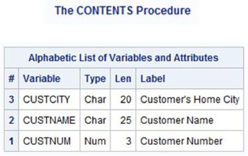
You should be aware that the SQL procedure ignores width specifications for numeric columns. When a numeric column is defined, it is created with a width of 8 bytes, which is the maximum precision allowed by SAS. PROC SQL ignores numeric length specifications when the value is less than 8 bytes. To illustrate this point, a partial CONTENTS procedure output is displayed for the CUSTOMERS table.

Results

To conserve storage space (CUSTNUM only requires maximum precision provided in 3 bytes), a LENGTH statement could be used in a DATA step to define CUSTNUM as a 3-byte column rather than an 8-byte column.

DATA Step Code

DATA CUSTOMERS;

  LENGTH CUSTNUM 3.;

  SET CUSTOMERS;

  LABEL CUSTNUM = ‘Customer Number’;

RUN;

Results

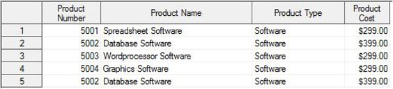
Let’s look at the column-definition list that is used to create the PRODUCTS table.

SQL Code

PROC SQL;

  CREATE TABLE PRODUCTS

    (PRODNUM   NUM(3)   LABEL=`Product Number’,

     PRODNAME  CHAR(25) LABEL=`Product Name’,

     MANUNUM   NUM(3)   LABEL=`Manufacturer Number’,

     PRODTYPE  CHAR(15) LABEL=`Product Type’,

     PRODCOST  NUM(5,2) FORMAT=DOLLAR9.2 LABEL=`Product Cost’);

QUIT;

SAS Log Results

The CONTENTS output for the PRODUCTS table shows once again that the SQL procedure ignores all width specifications for numeric columns.

Results

As before, to conserve storage space you can use a LENGTH statement in a DATA step to override the default 8-byte column definition for numeric columns.

DATA Step Code

DATA PRODUCTS;

  LENGTH PRODNUM MANUNUM 3.

         PRODCOST 5.;

  SET PRODUCTS(DROP=PRODNUM MANUNUM PRODCOST);

  LABEL PRODNUM  = ‘Product Number’

        MANUNUM  = ‘Manufacturer Number’

        PRODCOST = ‘Product Cost’;

  FORMAT PRODCOST DOLLAR9.2;

RUN;

Results

Referencing an existing table in a CREATE TABLE statement is an effective way of creating a new table. In fact, it can be a great time-saver, because it prevents having to define each column one at a time as was shown with column-definition lists. The LIKE clause (in the CREATE TABLE statement) triggers the existing table’s structure to be copied to the new table minus any columns dropped with the KEEP= or DROP= data set (table) option. It copies the column names and attributes from the existing table structure to the new table structure. Using this method results in the creation of an empty table (without rows). To illustrate this method of creating a new table, a table called HOT_PRODUCTS will be created with the LIKE clause.

SQL Code

PROC SQL;

  CREATE TABLE HOT_PRODUCTS

    LIKE PRODUCTS;

QUIT;

SAS Log Results

As a result of executing the CREATE TABLE statement and the LIKE clause the new table contains zero rows of data but does include all the column definitions without any rows of data from an existing table and/or view.  What this means is that only the metadata (data describing data) is copied to the new table.  The particular definitions that are copied include: column names, data type, length, precision, label, informat, format, and so on.

The next example illustrates how to create a new table by selecting only the columns that you have an interest in. This method is not supported by the SQL ANSI standard. Suppose that you want three columns (PRODNAME, PRODTYPE, and PRODCOST) from the PRODUCTS table. The following code illustrates how the KEEP= data set (table) option can be used to accomplish this.

Note: Data sets can also be called tables.

SQL Code

PROC SQL;

  CREATE TABLE HOT_PRODUCTS(KEEP=PRODNAME PRODTYPE PRODCOST)

    LIKE PRODUCTS;

QUIT;

 

SAS Log Results

Deriving a new table from an existing table is the most popular and effective way to create a table. This method uses a query expression, and the results are stored in a new table instead of being displayed as SAS output. This method not only stores the column names and their attributes, but also stores the rows of data that satisfy the query expression. The next example illustrates creating a new table with a query expression.

SQL Code

PROC SQL;

  CREATE TABLE HOT_PRODUCTS AS

    SELECT *

      FROM PRODUCTS;

QUIT;

SAS Log Results

You might notice after examining the SAS log in the previous example that the SELECT statement extracted all rows from the existing table (PRODUCTS) and copied them to the new table (HOT_PRODUCTS). In the absence of a WHERE clause, the resulting table (HOT_PRODUCTS) contains the identical number of rows as the parent table PRODUCTS.

The power of the CREATE TABLE statement, then, is in its ability to create a new table from an existing table. What is often overlooked in this definition is the CREATE TABLE statement’s ability to form a subset of a parent table. More frequently than not, a new table represents a subset of its parent table. For this reason, this method of creating a table is the most powerful and widely used. Suppose that you want to create a table called HOT_PRODUCTS that contains a subset of the “Software” and “Phones” product types. The following query-expression would accomplish this.

SQL Code

PROC SQL;

  CREATE TABLE HOT_PRODUCTS AS

    SELECT *

      FROM PRODUCTS

        WHERE UPCASE(PRODTYPE) IN (“SOFTWARE”, “PHONE”);

QUIT;

SAS Log Results

Let’s look at another example. Suppose that you want to create another table called NOT_SO_HOT_PRODUCTS that contains a subset of everything but the “Software” and “Phones” product types. The following query-expression would accomplish this.

SQL Code

PROC SQL;

  CREATE TABLE NOT_SO_HOT_PRODUCTS AS

    SELECT *

      FROM PRODUCTS

        WHERE UPCASE(PRODTYPE) NOT IN (“SOFTWARE”, “PHONE”);

QUIT;

SAS Log Results

After a table is created, it can then be populated with data. Unless the newly created table is defined as a subset of an existing table or its content is to remain static, one or more rows of data may eventually need to be added. The SQL standard provides the INSERT INTO statement as the vehicle for adding rows of data. In fact, the INSERT INTO statement doesn’t really insert rows of data at all. It simply adds each row to the end of the table.

The examples in this section look at a number of approaches to populate tables. As new rows of data are added to or changed in a target table, many things must be kept in-check behind the scenes including the need to carry out or commit any permanent changes to a table. This important step checks each write operation for errors and, should one or more errors occur, provides SAS with the ability to completely rollback or undo the changes since the last commit. For example, before a row insertion is allowed entry into a table with assigned integrity constraints, it is first marked as uncommitted, then validated against the assigned integrity constraints, and if no violations occur, the row insertion is committed to the table. The following row insertion methods are illustrated:

●         adding data to a table with a SET clause

●         adding data to all of the columns in a row

●         adding data to some of the columns in a row

●         adding data with a SELECT query

●         bulk loading data with Microsoft Excel

You populate tables with data by using an INSERT INTO statement. Three parameters are specified with an INSERT INTO statement: the name of the table, the names of the columns in which values are inserted, and the values themselves. One or more rows of data are inserted into a table with a SET clause. Suppose that you want to insert (or add) a single row of data to the CUSTOMERS table and the row consists of three columns (Customer Number, Customer Name, and Home City).

SQL Code

PROC SQL;

  INSERT INTO CUSTOMERS

     SET CUSTNUM=702,

         CUSTNAME=‘Mission Valley Computing’,

         CUSTCITY=‘San Diego’;

QUIT;

The SAS log displays the following message noting that one row was inserted into the CUSTOMERS table.

 

SAS Log Results

The inserted row of data from the INSERT INTO statement and SET clause is added to the end of the CUSTOMERS table.

Entering a new row into a table containing an index will automatically add the value to the index (for more information about indexes, see Chapter 6, “Modifying and Updating Tables and Indexes”). The following example illustrates adding three rows of data using the SET clause.

SQL Code

PROC SQL;

  INSERT INTO CUSTOMERS

    SET CUSTNUM=402,

        CUSTNAME=‘La Jolla Tech Center’,

        CUSTCITY=‘La Jolla’

    SET CUSTNUM=502,

        CUSTNAME=‘Alpine Byte Center’,

        CUSTCITY=‘Alpine’

    SET CUSTNUM=1702,

        CUSTNAME=‘Rancho San Diego Tech’,

        CUSTCITY=‘Rancho San Diego’;

QUIT;

The SAS log shows that three rows of data were inserted into the CUSTOMERS table.

SAS Log Results

The inserted rows of data from the INSERT INTO statement and SET clause are added to the end of the CUSTOMERS table.

Another way to populate a table with data uses a VALUES clause with an INSERT INTO statement. As described in the previous section, three parameters are specified with an INSERT INTO statement and a VALUES clause: the name of the table, the names of the columns in which values are inserted, and the values themselves. Data values are inserted into a table with a VALUES clause. Suppose that you want to insert (or add) a single row of data to the CUSTOMERS table, and the row consists of three columns (Customer Number, Customer Name, and Home City).

SQL Code

PROC SQL;

  INSERT INTO CUSTOMERS (CUSTNUM, CUSTNAME, CUSTCITY)

     VALUES (703, ‘Sonic Boom Analytics’, ‘Spring Valley’);

QUIT;

The SAS log displays the following message noting that one row was inserted into the CUSTOMERS table.

SAS Log Results

The inserted row of data from the previous INSERT INTO statement is added to the end of the CUSTOMERS table.

Entering a new row into a table that contains an index will automatically add the value to the index (for more information about indexes, see Chapter 6, “Modifying and Updating Tables and Indexes”). The INSERT INTO statement can also add multiple rows of data to a table. The following example illustrates adding three rows of data using the VALUES clause.

SQL Code

PROC SQL;

  INSERT INTO CUSTOMERS

            (CUSTNUM, CUSTNAME, CUSTCITY)

    VALUES (402, ‘La Jolla Tech Center’, ‘La Jolla’)

    VALUES (502, ‘Alpine Byte Center’,   ‘Alpine’)

    VALUES (1702,‘Rancho San Diego Tech’,‘Rancho San Diego’);

  SELECT *

    FROM CUSTOMERS

      ORDER BY CUSTNUM;

QUIT;

 

The SAS log shows three rows of data were inserted into the CUSTOMERS table.

SAS Log Results

The new rows are displayed in ascending order by CUSTNUM.

The INSERT INTO statement can also be used to insert rows of data without having to specify the column names as long as a value is keyed for each and every column in the table in the exact order that columns are specified in the table. Note: Learning the order of a table’s columns may require producing output from the CONTENTS procedure, and/or inspection of the metadata column, VARNUM, from the Dictionary.columns table or SASHELP.VCOLUMNS view.  The following example illustrates the absence of the table’s column names in the INSERT INTO statement as three rows of data are added using the VALUES clause.

SQL Code

PROC SQL;

  INSERT INTO CUSTOMERS

    VALUES (402, ‘La Jolla Tech Center’, ‘La Jolla’)

    VALUES (502, ‘Alpine Byte Center’,   ‘Alpine’)

    VALUES (1702,‘Rancho San Diego Tech’,‘Rancho San Diego’);

  SELECT *

    FROM CUSTOMERS

      ORDER BY CUSTNUM;

QUIT;

The SAS log shows three rows of data were inserted into the CUSTOMERS table.

SAS Log Results

The new rows are displayed in ascending order by CUSTNUM.

 

It is not uncommon when adding rows of data to a table to have one or more columns with an unassigned value. When this happens, SQL must be able to handle adding the rows to the table as if all of the values were present. But how does SQL handle values that are not specified? You will see in the following example that SQL assigns missing values to columns that do not have a value specified. As before, three parameters are specified with the INSERT INTO statement: the name of the table, the names of the columns in which values are inserted, and the values themselves. Suppose that you had to add two rows of incomplete data to the CUSTOMERS table, where two of three columns were specified (Customer Number and Customer Name).

SQL Code

PROC SQL;

  INSERT INTO CUSTOMERS

            (CUSTNUM, CUSTNAME)

     VALUES (102, ‘La Mesa Byte & Floppy’)

     VALUES (902, ‘Del Mar Technology Center’);

  SELECT *

    FROM CUSTOMERS

      ORDER BY CUSTNUM;

QUIT;

The SAS log shows that two rows of data were added to the CUSTOMERS table.

SAS Log Results

The new rows are displayed in ascending order by CUSTNUM with missing values assigned to the character column CUSTCITY.

In the previous example, missing values were assigned to the character column CUSTCITY. Suppose that you want to add two rows of partial data to the PRODUCTS table, where four of the five columns are specified (Product Number, Product Name, Product Type, and Product Cost), and the missing value for each row is the numeric column MANUNUM.

SQL Code

PROC SQL;

  INSERT INTO PRODUCTS

            (PRODNUM, PRODNAME, PRODTYPE, PRODCOST)

   VALUES(6002,'Security Software','Software',375.00)

   VALUES(1701,'Travel Laptop SE', 'Laptop',  4200.00);

  SELECT *

    FROM PRODUCTS

      ORDER BY PRODNUM;

QUIT;

The SAS log shows that two rows of data were added to the PRODUCTS table.

SAS Log Results

The new rows are displayed in ascending order by PRODNUM with missing values assigned to the numeric column MANUNUM.

You can also add data to a table using a SELECT query with an INSERT INTO statement. A query expression essentially executes an enclosed query by first creating a temporary table and then inserting the contents of the temporary table into the target table being populated. In the process of populating the target table, any columns omitted from the column list are automatically assigned to missing values.

In the next example, a SELECT query is used to add a row of data from the PRODUCTS table into the SOFTWARE_PRODUCTS table. The designated query controls the insertion of data into the target SOFTWARE_PRODUCTS table by using a WHERE clause.

SQL Code

PROC SQL;

  INSERT INTO SOFTWARE_PRODUCTS

             (PRODNUM, PRODNAME, PRODTYPE, PRODCOST)

    SELECT PRODNUM, PRODNAME, PRODTYPE, PRODCOST

      FROM PRODUCTS

        WHERE PRODTYPE IN (‘Software’) AND

              PRODCOST > 300;

QUIT;

The SAS log shows that one row of data was added to the SOFTWARE_PRODUCTS table.

SAS Log Results

The inserted row of data from the previous INSERT INTO statement is added to the end of the SOFTWARE_PRODUCTS table.

Although no specific SQL procedure statement or clause is available for bulk loading large amounts of data into a table, techniques for processing bulk load operations include using the IMPORT procedure, comma separated values (CSV) files, or LIBNAME statement with the Excel engine to populate tables. During the process of populating the target table, any columns omitted from the bulk load are automatically assigned to missing values.

In the next example, the IMPORT procedure is used to access and read data from the Excel file, PURCHASES.xls, and to create the SAS table, PURCHASES. The REPLACE option is specified to replace the PURCHASES table if it already exists. The Excel spreadsheet file appears below.

Table 5.1: PURCHASES Excel File

SQL Code

PROC IMPORT FILE=‘PURCHASES.XLS’

             OUT=PURCHASES

            DBMS=EXCEL

            REPLACE;

RUN;

The SAS log shows that 57 rows of data were imported from the PURCHASES spreadsheet.

SAS Log Results

 

The PURCHASES SAS table after being imported appears below.

Table 5.2: PURCHASES SAS Table

The IMPORT procedure can also be used to access and read comma separated values (CSV) files to populate SAS tables. In the next example, the PURCHASES CSV file, PURCHASES.csv, is read to populate the SAS table, PURCHASES. The DBMS=CSV option is specified to indicate that a CSV file is to be read, and the REPLACE option allows the PURCHASES table to be replaced if it already exists.

SQL Code

PROC IMPORT FILE=‘PURCHASES.CSV’

             OUT=PURCHASES

            DBMS=CSV

            REPLACE;

RUN;

The SAS log shows that 57 rows of data were imported from the PURCHASES CSV file.

SAS Log Results

SAS can also access and read Excel spreadsheet files with a LIBNAME statement. This allows worksheet files in an Excel file to be processed in much the same way as SAS data sets are processed in a SAS library. The general syntax for the LIBNAME statement using the EXCEL engine follows:

LIBNAME  libref  EXCEL  ‘spreadsheet-file-name.XLS’;

The libref is the library reference just as if you would use with a SAS data library. EXCEL is the name of the engine to use. The spreadsheet-file-name refers to the Excel file to use. The next example illustrates assigning the Excel LIBNAME engine to perform a bulk-load insert of the PURCHASES spreadsheet file into the PURCHASES table with the SQL procedure. Note: A separate SAS/ACCESS software for PC files license is required to use the Excel libname engine.

SQL Code

LIBNAME MYEXCEL EXCEL ‘PURCHASES.XLS’;

 

PROC SQL;

  INSERT INTO PURCHASES

    SELECT *

      FROM MYEXCEL.PURCHASES;

QUIT;

The SAS log shows that 57 rows of data were inserted into the WORK.PURCHASES table from the PURCHASES spreadsheet using the Excel LIBNAME engine.

SAS Log Results

The reliability of databases and the data within them is essential to every organization. Decision-making activities depend on the correctness and accuracy of any and all data contained in key applications, information systems, databases, decision support and query tools, as well as other critical systems. Even the slightest hint of unreliable data can affect decision-making capabilities, accuracy of reports, and, in those worst case scenarios, loss of user confidence in the database environment itself.

Because data should be correct and free of problems, an integral part of every database environment is a set of rules that the data should adhere to. These rules, often referred to as database-enforced constraints, are applied to the database table structure itself and determine the type and content of data that is permitted in columns and tables.

By implementing database-enforced integrity constraints, you can dramatically reduce data-related problems and additional programming work in applications. Instead of coding complex data checks and validations in individual application programs, you can build database-enforced constraints into the database itself. This work can eliminate the propagation of column duplication, invalid and missing values, lost linkages, and other data-related problems.

You define integrity constraints by specifying column definitions and constraints at the time a table is created with the CREATE TABLE statement, or by adding, changing, or removing a table’s column definitions with the ALTER TABLE statement. The rows in a table are then validated against the defined integrity constraints.

The first type of integrity constraint is referred to as a column and table constraint. This type of constraint essentially establishes rules that are attached to a specific table or column. The type of constraint is generally specified through one or two clauses with their distinct values as follows.

Column and Table Constraints

●         NOT NULL

●         UNIQUE

●         CHECK

A null value is essentially a missing or unknown value in the data. When unchecked, null values can often propagate themselves throughout a database. When a NULL appears in a mathematical equation, the returned result is also a null or missing value. When a NULL is used in a comparison or a logical expression, the returned result is unknown. The occurrence of null values presents problems during search, joins, and index operations. The ability to prevent the propagation of null values in a column with a NOT NULL constraint is a powerful feature of the SQL procedure. This constraint should be used as a first line of defense against potential problems that result from the presence of null values and the interaction of queries processing data.

Using the CREATE TABLE or ALTER TABLE statement, you can apply a NOT NULL constraint to any column where missing, unknown, or inappropriate values appear in the data. Suppose that you need to avoid the propagation of missing values in the CUSTCITY (Customer’s Home City) column in the CUSTOMER_CITY table. By specifying the NOT NULL constraint for the CUSTCITY column in the CREATE TABLE statement, you prevent the propagation of null values in a table.

SQL Code

PROC SQL;

  CREATE TABLE CUSTOMER_CITY

     (CUSTNUM NUM,

      CUSTCITY CHAR(20) NOT NULL);

QUIT;

Once the CUSTOMER_CITY table is created and the NOT NULL constraint is defined for the CUSTCITY column, only non-missing data for the CUSTCITY column can be entered. Using the INSERT INTO statement with a VALUES clause, you can populate the CUSTOMER_CITY table while adhering to the assigned NOT NULL integrity constraint.

SQL Code

PROC SQL;

  INSERT INTO CUSTOMER_CITY

    VALUES(101,`La Mesa Computer Land’)

    VALUES(1301,`Spring Valley Byte Center’);

QUIT;

The SAS log shows the two rows of data that satisfy the NOT NULL constraint, and the rows successfully being added to the CUSTOMER_CITY table.

SAS Log Results

When you define a NOT NULL constraint and then attempt to populate a table with one or more missing data values, the rows will be rejected and the table will be restored to its original state. Essentially, the insert fails because the NOT NULL constraint prevents any missing values for a defined column from populating a table. In the next example, several rows of data with a defined NOT NULL constraint are prevented from being populated in the CUSTOMER_CITY table because one row contains a missing CUSTCITY value.

SQL Code

PROC SQL;

  INSERT INTO CUSTOMER_CITY

    VALUES(101,’La Mesa Computer Land’)

    VALUES(1301,’Spring Valley Byte Center’)

    VALUES(1801,’’);

QUIT;

The SAS log shows that the NOT NULL constraint has prevented the three rows of data from being populated in the CUSTOMER_CITY table. The violation caused an error message that resulted in the failure of the add/update operation. The UNDO_POLICY = REQUIRED option reverses all adds/updates that have been performed to the point of the error. This prevents errors or partial data from being propagated in the database table. The following SAS log results illustrate the error condition that caused the add/update operation to fail.

SAS Log Results

A NOT NULL constraint can also be applied to a column in an existing table that contains data with an ALTER TABLE statement. To successfully impose a NOT NULL constraint, you should not have missing or null values in the column that the constraint is being defined for. This means that the presence of one or more null values in an existing table’s column will prevent the NOT NULL constraint from being created.

Suppose that the CUSTOMERS table contains one or more missing values in the CUSTCITY column. If you tried to add a NOT NULL constraint, it would be rejected. You can successfully apply the NOT NULL constraint only when missing values are reclassified or recoded.

SQL Code

PROC SQL;

  ALTER TABLE CUSTOMERS

    ADD CONSTRAINT NOT_NULL_CUSTCITY NOT NULL(CUSTCITY);

QUIT;

The SAS log shows that the NOT NULL constraint cannot be defined in an existing table when a column’s data contains one or more missing values. The violation produces an error message that results in the rejection of the constraint.

 

SAS Log Results

A UNIQUE constraint prevents duplicate values from propagating in a table. If you use a CREATE TABLE statement, then you can apply a UNIQUE constraint to any column where duplicate data is not desired. Suppose that you want to avoid the propagation of duplicate values in the CUSTNUM (Customer Number) column in a new table called CUSTOMER_CITY. By specifying the UNIQUE constraint for the CUSTNUM column with the CREATE TABLE statement, you prevent duplicate values from populating the table.

SQL Code

PROC SQL;

  CREATE TABLE CUSTOMER_CITY

     (CUSTNUM NUM UNIQUE,

      CUSTCITY CHAR(20));

QUIT;

When you define a UNIQUE constraint and attempt to populate a table with duplicate data values, the rows will be rejected and the table will be restored to its original state prior to the add operation taking place. Essentially, the insert fails because the UNIQUE constraint prevents any duplicate values for a defined column from populating the table. In the next example, several rows of data with a defined UNIQUE constraint are prevented from being populated in the CUSTOMER_CITY table because one row contains a duplicate CUSTNUM value.

SQL Code

PROC SQL;

  INSERT INTO CUSTOMER_CITY

    VALUES(101,’La Mesa Computer Land’)

    VALUES(1301,’Spring Valley Byte Center’)

    VALUES(1301,’Chula Vista Networks’);

QUIT;

The SAS log shows that the UNIQUE constraint prevented the three rows of data from being populated in the CUSTOMER_CITY table. The violation caused an error message that resulted in the failure of the add/update operation.

SAS Log Results

A CHECK constraint validates data values against a list of values, minimum and maximum values, as well as a range of values before populating a table. Using either a CREATE TABLE or ALTER TABLE statement, you can apply a CHECK constraint to any column that requires data validation to be performed. In the next example, suppose you want to validate data values in the PRODTYPE (Product Type) column in the PRODUCTS table. When you specify a CHECK constraint against the PRODTYPE column using the ALTER TABLE statement, product type values will first need to match the list of defined values or the rows will be rejected.

SQL Code

PROC SQL;

  ALTER TABLE PRODUCTS

    ADD CONSTRAINT CHECK_PRODUCT_TYPE

      CHECK (PRODTYPE IN (‘Laptop’,

                          ‘Phone’,

                          ‘Software’,

                          ‘Workstation’));

QUIT;

With a CHECK constraint defined, each row must meet the validation rules that are specified for the column before the table is populated. If any row does not pass the validation checks based on the established validation rules, then the add/update operation fails and the table is automatically restored to its original state prior to the operation taking place. In the next example, three rows of data are validated against the defined CHECK constraint established for the PRODTYPE column.

SQL Code

PROC SQL;

  INSERT INTO PRODUCTS

    VALUES(5005,’Internet Software’,500,’Software’,99.)

    VALUES(1701,’Elite Laptop’,170,’Laptop’,3900.)

    VALUES(2103,’Digital Cell Phone’,210,’Fone’,199.);

QUIT;

The SAS log displays the results after attempting to add the three rows of data. Because one row violates the CHECK constraint with a value of “Fone”, the rows are not added to the PRODUCTS table. The violation produces an error message that results in the failure of the add/update operation.

SAS Log Results

The second type of constraint that is available in the SQL procedure is referred to as a referential integrity constraint. Enforced through primary and foreign keys between two or more tables, referential integrity constraints are built into a database environment to prevent data integrity issues from occurring. Specific types of referential integrity constraints and constraint action clauses are used to enforce update and delete operations and consist of the following:

Referential Integrity Constraints

●         Primary key

●         Foreign key

Referential Integrity Constraint Action Clauses

●         RESTRICT (Default)

●         SET NULL

●         CASCADE

The action clauses are discussed in the “Establishing a Foreign Key” section in this chapter.

A primary key consists of one or more columns with a unique value that is used to identify individual rows in a table. Depending on the nature of the columns used, a single column may be all that is necessary to identify specific rows. In other cases, two or more columns may be needed to adequately identify a row in a referenced table. Suppose that you need to uniquely identify specific rows in the MANUFACTURERS table. By establishing the Manufacturer Number (MANUNUM) as the unique identifier for rows, a key is established. The next example specifies the ALTER TABLE statement to create a primary key using MANUNUM in the MANUFACTURERS table.

SQL Code

PROC SQL;

  ALTER TABLE MANUFACTURERS

    ADD CONSTRAINT PRIM_KEY PRIMARY KEY (MANUNUM);

QUIT;

The SAS log shows that the MANUFACTURERS table has been modified successfully after creating a primary key using the MANUNUM column.

SAS Log Results

Suppose that you also need to uniquely identify specific rows in the PRODUCTS table. By specifying PRODNUM (Product Number) as the primary key, the next example specifies the ALTER TABLE statement to create the unique identifier for rows in the table.

SQL Code

PROC SQL;

  ALTER TABLE PRODUCTS

    ADD CONSTRAINT PRIM_PRODUCT_KEY PRIMARY KEY (PRODNUM);

QUIT;

The SAS log shows that the PRODUCTS table has been modified successfully after establishing a primary key using the PRODNUM column.

SAS Log Results

A foreign key consists of one or more columns in a table that references or relates to values in another table. The column(s) that is used as a foreign key must match the column(s) in the table that is referenced. The purpose of a foreign key is to ensure that rows of data in one table exist in another table thereby preventing the possibility of lost or missing linkages between tables. The enforcement of referential integrity rules has a positive and direct effect on data reliability issues.

Suppose that you want to ensure that data values in the INVENTORY table have corresponding and matching data values in the PRODUCTS table. By establishing PRODNUM (Product Number) as a foreign key in the INVENTORY table, you ensure a strong level of data integrity between the two tables. This essentially verifies that key data in the INVENTORY table exists in the PRODUCTS table. In the next example, a foreign key is created using the PRODNUM column in the INVENTORY table by specifying the ALTER TABLE statement.

SQL Code

PROC SQL;

 ALTER TABLE INVENTORY

  ADD CONSTRAINT FOREIGN_PRODUCT_KEY FOREIGN KEY (PRODNUM)  

   REFERENCES PRODUCTS

    ON DELETE RESTRICT

    ON UPDATE RESTRICT;

QUIT;

The SAS log displays the successful creation of the PRODNUM column as a foreign key in the INVENTORY table. By specifying the default values ON DELETE RESTRICT and ON UPDATE RESTRICT clauses, you restrict the ability to change the values of primary key data when matching values are found in the foreign key. The execution of any SQL statement that could violate these referential integrity rules is prevented during SQL processing.

 

SAS Log Results

Suppose that a product of a particular manufacturer is no longer available and has been taken off the market. To handle this type of situation, data values in the INVENTORY table should be set to missing once the product is deleted from the PRODUCTS table. The next example establishes a foreign key using the PRODNUM column in the INVENTORY table and sets values to null with the ON DELETE clause.

SQL Code

PROC SQL;

 ALTER TABLE INVENTORY

  ADD CONSTRAINT FOREIGN_MISSING_PRODUCT_KEY FOREIGN KEY (PRODNUM)  

   REFERENCES PRODUCTS

    ON DELETE SET NULL;

QUIT;

The SAS log displays the successful creation of the PRODNUM column as a foreign key in the INVENTORY table as well as the effect of the ON DELETE SET NULL clause. Specifying this clause will change foreign key values to missing or null for all of the rows with matching values found in the primary key. The execution of any SQL statement that could violate these referential integrity rules is prevented during SQL processing.

SAS Log Results

Suppose that you want to ensure that changes to key values in the PRODUCTS table automatically flow over or cascade through to rows in the INVENTORY table. This is accomplished by first creating PRODNUM (Product Number) as a foreign key in the INVENTORY table using the ADD CONSTRAINT clause and referencing the PRODUCTS table. You then specify the ON UPDATE CASCADE clause to enable any changes that are made to the PRODUCTS table to be automatically cascaded through to the INVENTORY table. This ensures that changes to the product number values in the PRODUCTS table automatically occur in the INVENTORY table as well.

SQL Code

PROC SQL;

 ALTER TABLE INVENTORY

  ADD CONSTRAINT FOREIGN_PRODUCT_KEY FOREIGN KEY (PRODNUM)  

   REFERENCES PRODUCTS

    ON UPDATE CASCADE

    ON DELETE RESTRICT  /* DEFAULT VALUE */;

QUIT;

The SAS log displays the successful creation of the PRODNUM column as a foreign key in the INVENTORY table. When the ON UPDATE and ON DELETE clauses are specified, the execution of any SQL statement that could violate referential integrity rules is strictly prohibited.

SAS Log Results

Constraints and Change Control

To preserve change control, SAS prohibits changes or modifications to a table that contains a defined referential integrity constraint. When you attempt to delete, rename, or replace a table that contains a referential integrity constraint, an error message is generated and processing stops. The next example illustrates a table copy operation that is performed against a table that contains a referential integrity constraint that generates an error message and stops processing.

SAS Log Results

Using the DESCRIBE TABLE statement, the SQL procedure displays integrity constraints along with the table description in the SAS log. The ability to capture this type of information assists with the documentation process by describing the names and types of integrity constraints as well as the contributing columns that they reference.

SQL Code

PROC SQL;

  DESCRIBE TABLE MANUFACTURERS;

QUIT;

The SAS log shows the SQL statements that were used to create the MANUFACTURERS table as well as an alphabetical list of integrity constraints that have been defined.

SAS Log Results

In the world of data management, the ability to delete unwanted rows of data from a table is as important as being able to populate a table with data. In fact, data management activities would be severely hampered without the ability to delete rows of data. The DELETE statement and an optional WHERE clause can remove one or more unwanted rows from a table, depending on what is specified in the WHERE clause.

The DELETE statement can be specified to remove a single row of data by constructing an explicit WHERE clause on a unique value. The construction of a WHERE clause to satisfy this form of row deletion may require a complex logic construct. So, be sure to test the expression thoroughly before applying it to the table to determine whether it performs as expected. The following example illustrates the removal of a single customer in the CUSTOMERS table by specifying the customer’s name (CUSTNAME) in the WHERE clause.

SQL Code

PROC SQL;

  DELETE FROM CUSTOMERS2

    WHERE UPCASE(CUSTNAME) = “LAUGHLER”;

QUIT;

SAS Log Results

Frequently, a row deletion affects more than a single row in a table. In these cases, a WHERE clause references a value that occurs multiple times. The following example illustrates the removal of a single customer in the PRODUCTS table by specifying the product type (PRODTYPE) in the WHERE clause.

SQL Code

PROC SQL;

  DELETE FROM PRODUCTS

    WHERE UPCASE(PRODTYPE) = `PHONE’;

QUIT;

 

SAS Log Results

SQL provides a simple way to delete all rows in a table. The following example shows that all rows in the CUSTOMERS table can be removed when the WHERE clause is omitted. Use care when using this form of the DELETE statement because every row in the table is automatically deleted.

SQL Code

PROC SQL;

  DELETE FROM CUSTOMERS;

QUIT;

SAS Log Results

The SQL standard permits one or more unwanted tables to be removed (or deleted) from a database (SAS library). During large program processes, temporary tables in the WORK library are frequently created. The creation and build-up of these tables can negatively affect memory and storage performance areas, which can cause potential problems due to insufficient resources. It is important from a database management perspective to be able to delete any unwanted tables to avoid these types of resource problems. Here are a few guidelines to keep in mind.

Before a table can be deleted, complete ownership of the table (that is, exclusive access to the table) should be verified. Although some SQL implementations require a table to be empty in order to delete it, the SAS implementation permits a table to be deleted with or without any rows of data in it. After a table is deleted, any references to that table are no longer recognized and will result in a syntax error. Additionally, any references to a deleted table in a view will also result in an error (see Chapter 8, “Working with Views”). Also, any indexes that are associated with a deleted table are automatically dropped (see Chapter 6, “Modifying and Updating Tables and Indexes”).

Deleting a table from the database environment is not the same as making a table empty. Although an empty table contains no data, it still possesses a structure; a deleted table contains no data or related structure. Essentially, a deleted table does not exist because the table including its data and structure are physically removed forever. Deleting a single table from a database environment requires a single table name to be referenced in a DROP TABLE statement. In the next example, a single table called HOT_PRODUCTS located in the WORK library is physically removed using a DROP TABLE statement.

SQL Code

PROC SQL;

  DROP TABLE HOT_PRODUCTS;

QUIT;

SAS Log Results

The SQL standard also permits more than one table to be specified in a single DROP TABLE statement. The next example and corresponding log shows two tables (HOT_PRODUCTS and NOT_SO_HOT_PRODUCTS) being deleted from the WORK library.

SQL Code

PROC SQL;

  DROP TABLE HOT_PRODUCTS, NOT_SO_HOT_PRODUCTS;

QUIT;

SAS Log Results

As previously discussed in this chapter, to ensure a high-level of data integrity in a database environment, the SQL standard permits the creation of one or more integrity constraints to be imposed on a table. Under the SQL standard, a table that contains one or more constraints cannot be deleted without first dropping the defined constraints. This behavior further safeguards and prevents the occurrence of unanticipated surprises such as the accidental deletion of primary or supporting tables.

In the next example, the SAS log shows that an error is produced when an attempt to drop a table containing an ON DELETE RESTRICT referential integrity constraint is performed. The referential integrity constraint causes the DROP TABLE statement to fail, which results in the INVENTORY table not being deleted.

SAS Log Results

To enable the deletion of a table that contains one or more integrity constraints, you must specify an SQL statement such as the ALTER TABLE statement and DROP COLUMN or DROP CONSTRAINT clauses. Once a table’s integrity constraints are removed, the table can then be deleted.

In the following SAS log, the FOREIGN_PRODUCT_KEY constraint is removed from the INVENTORY table using the DROP CONSTRAINT clause. With the constraint removed, the INVENTORY table is then deleted with the DROP TABLE statement.

SAS Log Results

 

1.       Creating a table using a column-definition list is similar to defining a table’s structure with the LENGTH statement in the DATA step (see the “Creating a Table Using Column-Definition Lists section).

2.       Using the LIKE clause copies the column names and attributes from the existing table structure to the new table structure (see the “Creating a Table Using the LIKE Clause section).

3.       Deriving a table from an existing table stores the results in a new table instead of displaying them as SAS output (see the “Deriving a Table and Data from an Existing Table” section).

4.       In populating a table, three parameters are specified with an INSERT INTO statement: the name of the table, the names of the columns in which values are inserted, and the values themselves (see the “Adding Data to All of the Columns in a Row” section).

5.       Database-enforced constraints can be applied to a database table structure to enforce the type and content of data that is permitted (see the “Integrity Constraints” section).

6.       The DELETE statement combined with a WHERE clause selectively removes one or more rows of data from a table (see the “Deleting a Single Row in a Table” section).

7.       The SQL standard permits one or more unwanted tables to be removed from a database (SAS library) (see the “Deleting Multiple Tables” section).