
Chapter 4: Coding PROC SQL Logic
Conditional Logic with Predicates (Operators)
Case Logic versus COALESCE Expression
Assigning Labels and Grouping Data
Interfacing PROC SQL with the Macro Language
Exploring Macro Variables and Values
Creating Multiple Macro Variables
Using Automatic Macro Variables to Control Processing
Building Macro Tools and Applications
Determining the Number of Rows in a Table
Identifying Duplicate Rows in a Table
Expressions in the SQL procedure can be simple or complex and are represented by a combination of columns, symbols, operators, functions, constants, and literals. Specified in SQL statements and clauses, expressions are typically used in conditional logic constructs to test or compare a value against another value. The application of an expression in a CASE expression allows individual rows of data to be processed and grouped using one or more expressions. In particular, data can be recoded and reshaped to expand the data analysis and processing perspective.
As experienced PROC SQL programmers know, it is often necessary to test and evaluate conditions as true or false. From a programming perspective, the evaluation of a condition determines which of the alternate paths a program will follow. Conditional logic for selecting rows in one or more tables in the SQL procedure is most frequently specified using a WHERE or ON clause, or a WHERE or HAVING clause, to reference constants and relationships among columns, values, or aggregates. Essentially, a WHERE, ON, or HAVING clause along with its associated expression defines a condition for selecting rows or aggregates from one or more tables.
The SQL procedure also allows the identification and assignment of data values in a SELECT statement using CASE expressions (which are described in the next section). To show how constants and relationships are referenced in a WHERE clause, a number of examples will be presented including a single column (variable) name or constant, a SAS function, a predicate, and a compound expression consisting of a series of simple expressions.
Conversations frequently arise about whether a WHERE clause or an ON clause should be specified when a query performs a join on two or more tables. Here is a brief and simple explanation of what happens when a WHERE clause is specified versus an ON clause in a join query.
A join query containing a WHERE clause results in SAS performing the filtering operation after the tables have been joined. For example, when a conventional inner join operation containing a WHERE clause is executed the tables are first joined, and then filtered, followed by the results being produced. You are asked to contrast these operations with a join query that contains an ON clause. A join query containing an ON clause results in one or both of the tables being filtered prior to being joined. As a result, the flow of operations when a WHERE clause is specified differs from when an ON clause is specified in a join query.
When specified, the optional WHERE and HAVING clause applies subsetting conditions on the rows selected from the table(s) specified in the FROM clause. A WHERE clause is specified to process rows of data using any valid SAS expression, the specification of an aggregate (e.g., COUNT, MIN, MAX, etc.) is not allowed. To process aggregated data, a HAVING clause is specified in place of a WHERE clause. Note: As was described in Chapter 2, “Working with Data in PROC SQL,” a WHERE clause is specified before a GROUP BY clause (pre-filter), and a HAVING clause is specified after a GROUP BY clause (post-filter).
The next example shows a WHERE clause subsetting products from the PRODUCTS table that cost less than $400.00. During execution, the expression evaluates to true when the value of PRODCOST is less than $400.00. Otherwise, when the value of PRODCOST is greater than or equal to $400.00, the expression evaluates to false. This is an important concept because data rows are only selected when the WHERE clause expression evaluates to true.
SQL Code
PROC SQL;
SELECT *
FROM PRODUCTS
WHERE PRODCOST < 400.00;
QUIT;
In the next example, the following relation evaluates whether the cost of a product (PRODCOST) is greater than $400.00. When the WHERE clause expression evaluates to true, which means that PRODCOST is greater than $400.00, then the rows of data are selected. Otherwise, when the value is less than or equal to $400.00, the expression evaluates to false.
SQL Code
PROC SQL;
SELECT *
FROM PRODUCTS
WHERE PRODCOST > 400.00;
QUIT;
A relation can also be used with nonnumeric literals and nonnumeric columns. In the next example, a case-sensitive expression is constructed to represent the type of product (PRODTYPE) made by a manufacturer. When evaluated, a condition of true or false is produced depending on whether the current value of PRODTYPE is identical (character-by- character) to the literal value “Software”. When a condition of true occurs, then the rows of data satisfying the expression are selected; otherwise, they are not selected.
SQL Code
PROC SQL;
SELECT *
FROM PRODUCTS
WHERE PRODTYPE = “Software”;
QUIT;
To ensure a character-by-character match of a character value, the previous expression could be specified in a WHERE clause with the UPCASE function as follows.
SQL Code
PROC SQL;
SELECT *
FROM PRODUCTS
WHERE UPCASE(PRODTYPE) = “SOFTWARE”;
QUIT;
The previous query’s conditional expression could also be specified in a HAVING clause with the UPCASE function as follows.
SQL Code
PROC SQL;
SELECT *
FROM PRODUCTS
HAVING UPCASE(PRODTYPE) = “SOFTWARE”;
QUIT;
When the relations < and > are defined for nonnumeric values, the issue of implementation-dependent collating sequence for characters comes into play. For example, “A” < “B” is true, “Y” < “Z” is “true”, “B” < “A” is “false”, and so on. For more information about character collating sequences, refer to your specific operating system documentation.
To continue contrasting the differences between a WHERE clause and a HAVING clause, the next example specifies a WHERE clause to count and subset the product types from the PRODUCTS table so that product types containing four or more products are displayed. As can be seen in the SAS log results, unfortunately, the SAS System stopped processing this query because the use of summary functions in a WHERE clause is not permitted.
SQL Code
PROC SQL;
SELECT PRODNAME
,PRODTYPE
,PRODCOST
FROM PRODUCTS
WHERE COUNT(PRODTYPE) > 3
GROUP BY PRODTYPE
ORDER BY PRODNAME;
QUIT;
SAS Log Results
PROC SQL;
SELECT PRODNAME
,PRODTYPE
,PRODCOST
FROM PRODUCTS
WHERE COUNT(PRODTYPE) > 3
GROUP BY PRODTYPE
ORDER BY PRODNAME;
ERROR: Summary functions are restricted to the SELECT and HAVING clauses only.
NOTE: PROC SQL set option NOEXEC and will continue to check the syntax of statements.
QUIT;
NOTE: The SAS System stopped processing this step because of errors.
To successfully count and subset products containing four or more product types, the next query replaces the WHERE clause in the previous example with a HAVING clause to avoid the restrictions noted earlier. As shown in the results, the products matching the post-filtering operation performed by the HAVING clause are selected and displayed without error.
SQL Code
PROC SQL;
SELECT PRODNAME
,PRODTYPE
,PRODCOST
FROM PRODUCTS
GROUP BY PRODTYPE
HAVING COUNT(PRODTYPE) > 3
ORDER BY PRODNAME;
QUIT;
Results

Conditional logic and the use of predicates (e.g., IN, BETWEEN, and CONTAINS) provide WHERE and HAVING clauses with added value and flexibility. In Hermansen and Legum (2008), the authors describe using predicates to perform complex table look-up, subsetting, and other operations. Predicates are used in WHERE and HAVING clauses when a Boolean value is necessary. From fully bounded range conditions, and operators such as IN, BETWEEN, and CONTAINS, predicates provide users with a way to streamline WHERE and HAVING clause expressions.
In the next example, a WHERE clause with an UPCASE function and an OR logical operator is constructed to select rows matching the literal value “LAPTOP” or “WORKSTATION”. When a condition of true occurs for either value, then the rows of data satisfying the expression are selected; otherwise, they are not selected.
SQL Code
PROC SQL;
SELECT *
FROM PRODUCTS
WHERE UPCASE(PRODTYPE) = “LAPTOP” OR UPCASE(PRODTYPE) = “WORKSTATION”;
QUIT;
However, an easier and more convenient way of specifying the WHERE clause in the previous example is to use an IN operator to select product types from the PRODUCTS table that match the list of character values, as follows.
SQL Code
PROC SQL;
SELECT *
FROM PRODUCTS
WHERE UPCASE(PRODTYPE) IN (“LAPTOP”, “WORKSTATION”);
QUIT;
In the next example, a WHERE clause specifies a fully bounded range condition that selects and orders products that cost between $200 and $400.
SQL Code
PROC SQL;
SELECT *
FROM PRODUCTS
WHERE 200 <= PRODCOST <= 400
ORDER BY PRODCOST, PRODNAME;
QUIT;
However, a more convenient way of specifying the WHERE clause in the previous example is to use a BETWEEN operator which selects and orders products from the PRODUCTS table that cost between $200 and $400, as follows.
SQL Code
PROC SQL;
SELECT *
FROM PRODUCTS
WHERE PRODCOST BETWEEN 200 AND 400
ORDER BY PRODCOST, PRODNAME;
QUIT;
Another handy operator to use in a WHERE or HAVING clause is CONTAINS. The CONTAINS operator selects rows by searching for a specified set of characters contained in a character variable. The next example selects the company names from the CUSTOMERS table that contain the characters “TECH” in the customer name, as follows.
SQL Code
PROC SQL;
SELECT *
FROM CUSTOMERS
WHERE UPCASE(CUSTNAME) CONTAINS “TECH”
ORDER BY CUSTNAME;
QUIT;
The next example shows how a NOT logical operator can be specified to select the company names from the CUSTOMERS table that do not contain the characters “TECH” in the customer name, as follows.
SQL Code
PROC SQL;
SELECT *
FROM CUSTOMERS
WHERE UPCASE(CUSTNAME) NOT CONTAINS “TECH”
ORDER BY CUSTNAME;
QUIT;
In the SQL procedure, a CASE expression provides a way of determining what the resulting value will be from all the rows in a table (or view). Similar to a DATA step SELECT statement (or IF‑THEN/ELSE statement), a CASE expression is based on some condition and the condition uses a WHEN-THEN clause to determine what the resulting value will be. An optional ELSE expression can be specified to handle an alternative action if none of the expression(s) identified in the WHEN condition(s) is satisfied.
The SQL procedure supports two forms of CASE expressions: simple and searched. CASE expressions can be specified in a SELECT clause, a WHERE clause, an ORDER BY clause, a HAVING clause, a join construct, and anywhere an expression can be used. A CASE expression must be a valid PROC SQL expression and conform to syntax rules similar to DATA step SELECT-WHEN statements. Before specific CASE expression examples are shown, it’s important to illustrate the basic syntax, which is shown below.
CASE <column-name>
WHEN when-condition THEN result-expression
<WHEN when-condition THEN result-expression> …
<ELSE result-expression>
END
The CASE syntax contains everything from CASE to END. A column-name can optionally be specified as part of the CASE expression. If present, it is automatically made available to each WHEN condition. When it is not specified, the column name must be coded in each WHEN condition. Let’s examine how a CASE expression works.
One or more WHEN conditions can be specified in a CASE expression and are evaluated in the order listed. If a WHEN condition is satisfied by a row in a table (or view), then it is considered “true” and the result expression following the THEN keyword is processed. The remaining WHEN conditions in the CASE expression are skipped. If a WHEN condition is “false,” the next WHEN condition is evaluated. SQL evaluates each WHEN condition until a “true” condition is found. Or, in the event that all WHEN conditions are “false,” it then executes the ELSE expression and assigns its value to the CASE expression’s result. A missing value is assigned to a CASE expression when an ELSE expression is not specified and each WHEN condition is “false.”
As its name implies, a simple CASE expression provides a useful way to perform the simplest type of comparisons. The syntax requires a column name from an underlying table to be specified as part of the CASE expression. This not only eliminates having to continually repeat the column name in each WHEN condition, it also reduces the number of keystrokes, making the code easier to read (and support). Simple CASE expressions possess the following features:
● Allows only equality checks.
● Evaluates the specified WHEN conditions in the order specified.
● Evaluates the input-expression for each WHEN condition.
● Returns the result-expression of the first input-expression that evaluates to “true.”
● If no input-expressions evaluate to “true,” then the ELSE condition is processed.
● When an ELSE condition isn’t specified, a NULL value is assigned.
Simple CASE Expression in a SELECT Clause
To best show how a simple CASE expression works, an example in a SELECT clause is illustrated. The objective calls for the value assignment of “East” to manufacturers in Florida, “Central” to manufacturers in Texas, “West” to manufacturers in California, or “Unknown” to manufacturers not residing in Florida, Texas, and California. The manufacturer’s state of residence (MANUSTAT) column is specified in the CASE expression along with its associated WHEN conditions with assigned values. Finally, a column heading of Region is assigned to the derived output column using the AS keyword.
SQL Code
PROC SQL;
SELECT MANUNAME,
MANUSTAT,
CASE MANUSTAT
WHEN 'CA' THEN 'West'
WHEN 'FL' THEN 'East'
WHEN 'TX' THEN 'Central'
ELSE 'Unknown'
END AS Region
FROM MANUFACTURERS;
QUIT;
Results

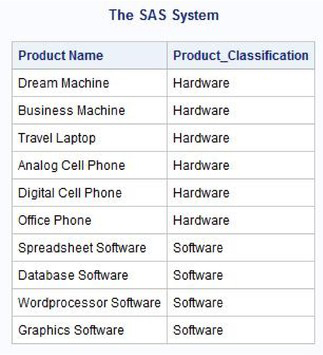
The next example illustrates the process of classifying products with a simple CASE expression in a SELECT clause. The PRODTYPE column from the PRODUCTS table is used to assign a character value of “Hardware,” “Software,” or “Unknown” to each product type (e.g., Laptop, Phone, Software, and Workstation). Similar to the assignment process in the FORMAT procedure, new data values are associated with values in the PRODTYPE column. The WHEN-THEN conditions equate “Laptop” to “Hardware,” “Phone” to “Hardware,” “Software” to “Software,” and “Workstation” to “Hardware.” A value of “Unknown” is assigned to products not matching any of the WHEN‑THEN logic conditions. Finally, a column heading of Product_Classification is assigned to the new column with the AS keyword.
SQL Code
PROC SQL;
SELECT PRODNAME,
CASE PRODTYPE
WHEN ‘Laptop’ THEN ‘Hardware’
WHEN ‘Phone’ THEN ‘Hardware’
WHEN ‘Software’ THEN ‘Software’
WHEN ‘Workstation’ THEN ‘Hardware’
ELSE ‘Unknown’
END AS Product_Classification
FROM PRODUCTS;
QUIT;
Results
The next example classifies products (e.g., Laptop/Workstation, Phone, and Software) in the PRODUCTS table using a simple CASE expression. A PUT function converts the numeric-defined PRODNUM column to a character value, and the SUBSTR function then extrapolates the first position in the PRODNUM column for classification purposes in the WHEN-THEN logic conditions. Finally, a column heading is assigned to the output column with the AS keyword.
SQL Code
PROC SQL;
SELECT PRODNAME,
PRODNUM,
CASE SUBSTR(PUT(PRODNUM,4.),1,1)
WHEN ‘1’ THEN ‘Laptop/Workstation’
WHEN ‘2’ THEN ‘Phone’
WHEN ‘5’ THEN ‘Software’
ELSE ‘Unknown’
END AS Product_Classification
FROM PRODUCTS
ORDER BY PRODNUM;
QUIT;
Results

The next example applies a subquery (for more information, see the “Subqueries” section in Chapter 7, “Coding Complex Queries”) to subset software products from the Product_Classification results created in the previous example.
SQL Code
PROC SQL;
SELECT *
FROM
(SELECT PRODNAME,
PRODNUM,
CASE SUBSTR(PUT(PRODNUM,4.),1,1)
WHEN ‘1’ THEN ‘Laptop/Workstation’
WHEN ‘2’ THEN ‘Phone’
WHEN ‘5’ THEN ‘Software’
ELSE ‘Unknown’
END AS Product_Classification
FROM PRODUCTS
)
WHERE Product_Classification = ‘Software’;
QUIT;
Results

Simple CASE Expression in a WHERE Clause
In the previous section, we examined the syntax and application of simple CASE expressions in a SELECT clause. In this section, we’ll explore the syntax and application of simple CASE expressions in a WHERE clause. Because the SQL procedure supports the use of a CASE expression anywhere an expression can be used, we’ll learn that a query can benefit from the capabilities of passing a result value from a CASE expression directly to a WHERE clause in place of a hardcoded value.
SQL Code
PROC SQL;
SELECT MANUNAME,
MANUSTAT
FROM MANUFACTURERS
WHERE CASE MANUSTAT
WHEN 'CA' THEN 1
ELSE 0
END;
QUIT;
Results
Creating a Customized List with a Simple CASE Expression
A customized display and order can be coded using a simple CASE expression in a SELECT and ORDER BY clause. The following example illustrates a unique way to create a list of products and availability by coding individual Case logic for each product in the PRODUCTS table. The resulting output displays a value of “1” to indicate that it contributed to the output list, or a value of “0” to indicate that it didn’t contribute to the output list.
SQL Code
OPTIONS LS=120;
PROC SQL;
SELECT PRODNAME,
PRODCOST,
CASE PRODTYPE WHEN 'Laptop' THEN 1 ELSE 0 END
AS LaptopRequest,
CASE PRODTYPE WHEN 'Workstation' THEN 1 ELSE 0 END
AS WorkstationRequest,
CASE PRODTYPE WHEN 'Phone' THEN 1 ELSE 0 END
AS PhoneRequest,
CASE PRODTYPE WHEN 'Software' THEN 1 ELSE 0 END
AS SoftwareRequest
FROM PRODUCTS
ORDER BY CASE PRODTYPE WHEN 'Laptop' THEN 1 ELSE 0 END,
CASE PRODTYPE WHEN 'Workstation' THEN 1 ELSE 0 END,
CASE PRODTYPE WHEN 'Phone' THEN 1 ELSE 0 END,
CASE PRODTYPE WHEN 'Software' THEN 1 ELSE 0 END;
QUIT;
Results

Simple CASE Expression in a HAVING Clause
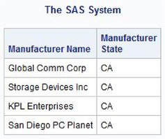
A HAVING clause is used in an SQL query to filter out aggregates specified in a GROUP BY clause. In this example, the SELECT clause returns the names of the manufacturers along with their state of residence from the MANUFACTURERS table. The CASE expression in the HAVING clause restricts what is returned by the SELECT clause to only the manufacturers residing in the state of California.
SQL Code
PROC SQL;
SELECT MANUNAME,
MANUSTAT
FROM MANUFACTURERS
HAVING CASE MANUSTAT
WHEN 'CA' THEN 1
ELSE 0
END;
QUIT;
Results

In the next example, the SELECT clause returns the most expensive product(s) from the PRODUCTS table, and the CASE expression in the HAVING clause restricts the results to software products costing more than $300.00.
SQL Code
PROC SQL;
SELECT PRODNAME,
PRODTYPE,
MAX(PRODCOST) AS Product_Cost FORMAT=DOLLAR10.2
FROM PRODUCTS
HAVING CASE PRODTYPE
WHEN 'Software' THEN PRODCOST
ELSE 0
END > 300;
QUIT;
Results

Simple CASE Expression in a Join Construct
A CASE expression can be specified in a JOIN construct to filter out aggregates specified in a GROUP BY clause. In this example, the SELECT clause returns the names of the manufacturers along with their state of residence from the MANUFACTURERS table. The CASE expression in the HAVING clause restricts what is returned by the SELECT clause to just the manufacturers residing in the state of California.
SQL Code
PROC SQL;
SELECT PRODNAME,
PRODTYPE,
MANUNAME
FROM PRODUCTS P,
MANUFACTURERS M
WHERE P.MANUNUM = M.MANUNUM AND
CASE PRODTYPE
WHEN 'Software' THEN 1
ELSE 0
END;
QUIT;
Results

Preventing Division by Zero with a Simple CASE Expression
Division by zero errors can cause many problems for a query, including severe performance degradation. In the next example, a simple CASE expression in a SELECT clause is specified to prevent division by zero errors. Using the INVENTORY table, a CASE expression tells SAS to ignore performing any computations for products containing an INVENQTY value of zero (by assigning a Boolean value of false). Otherwise, the equation INVENCST / INVENQTY is computed and products costing more than $1,000.00 are selected by the WHERE clause. A column heading called, Average_Cost is assigned to the new column with the AS keyword.
SQL Code
PROC SQL;
SELECT PRODNUM,
INVENQTY,
INVENCST,
CASE INVENQTY
WHEN 0 THEN 0
ELSE INVENCST / INVENQTY
END AS Average_Cost FORMAT=DOLLAR10.2
FROM INVENTORY
WHERE INVENCST / INVENQTY > 1000;
QUIT;
Results

In the next example, a simple CASE expression is implemented in a WHERE clause to prevent division by zero errors. As before, the CASE expression’s WHEN condition tells SAS to ignore performing any computations for products containing an INVENQTY value of zero (by assigning a Boolean value of false). Otherwise, the equation INVENCST / INVENQTY is computed and products costing more than $1,000.00 are selected by the WHERE clause.
SQL Code
PROC SQL;
SELECT PRODNUM,
INVENQTY,
INVENCST
FROM INVENTORY
WHERE CASE INVENQTY
WHEN 0 THEN 0
ELSE INVENCST / INVENQTY
END > 1000;
QUIT;
Results

Nesting Simple CASE Expressions
Much has been written on the techniques associated with software construction, particularly about aspects related to program and/or code design. When discussions of program complexity arise, it is widely accepted that a program’s degree of complexity can often be reduced by dividing its solution into smaller pieces or parts. This rule of thinking is perhaps best discussed in Steve McConnell’s book, Code Complete: A Practical Handbook of Software Construction, Second Edition (2004), “Humans tend to have an easier time comprehending several simple pieces of information than one complicated piece.”
Although many design strategies exist to improve the process of program design, one strategy frequently mentioned is the process of nesting. Nesting involves converting complex and/or cumbersome logic scenarios into two (or more) simpler logic conditions. The primary objective is to improve a program’s maintainability and readability. This rule of thought is further reinforced by the SQL procedure’s support for nesting using a CASE expression construct.
Nesting can be a useful technique because it provides SQL users with an effective way to handle complex code. But, unnecessary nesting or nesting just for the sake of nesting can actually make code more difficult to comprehend and maintain. It’s been my experience that nesting should never exceed three or four levels deep. Anything more than that and the degree of complexity can increase significantly. The general rule is to develop code that’s not only easy to understand, but hopefully contains fewer errors. To illustrate the process of nesting, a simple CASE expression is nested two levels deep for identifying software products in the PRODUCTS table that cost less than $300.00.
SQL Code
PROC SQL;
SELECT PRODNAME,
PRODTYPE,
PRODCOST,
CASE PRODTYPE
WHEN ‘Software’ THEN
CASE
WHEN PRODCOST < 300 THEN ‘Match’
ELSE ‘No Match’
END
ELSE ‘Not Software’
END AS Product_Type_Cost
FROM PRODUCTS;
QUIT;
Results

Conditionally Updating a Table with a Simple CASE Expression
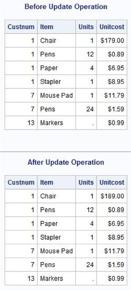
A CASE expression can be specified to conditionally update the contents of a table. For more information about updating data in a table, see Chapter 6, “Modifying and Updating Tables and Indexes.” The example illustrates the process of conditionally updating data in a table using an UPDATE statement and a simple CASE expression to add $10.00 the unit cost (UNITCOST) for a “Chair” in the PURCHASES table from $179.00 to $189.00.
Note: A table must be open in update mode to be able to update its contents.
SQL Code
PROC SQL;
TITLE1 ‘Before Update Operation’;
SELECT *
FROM PURCHASES2;
UPDATE PURCHASES2
SET UNITCOST = UNITCOST +
CASE ITEM
WHEN ‘Chair’ THEN 10.00
ELSE 0
END;
TITLE1 ‘After Update Operation’;
SELECT *
FROM PURCHASES2;
QUIT;
Results
A searched CASE expression provides SQL users with the capability to perform more complex comparisons. Although the number of keystrokes can be more than with a simple CASE expression, the searched CASE expression offers the greatest flexibility and is the primary form used by SQL programmers. The noticeable absence of a column name as part of the CASE expression permits any number of columns to be specified from the underlying table(s) in the WHEN‑THEN/ELSE logic scenarios.
The searched CASE expression evaluates one or more WHEN conditions until it encounters one that evaluates to “true.” It then assigns the corresponding result expression specified following the THEN keyword. If none of the WHEN conditions evaluates to “true,” then the result following the specified ELSE keyword is returned. If none of the WHEN conditions evaluates to “true” and an ELSE condition is not specified, then the searched CASE expression returns a null value. Searched CASE expressions possess the following features:
● Allow arithmetic operators (i.e., =, <, <=, >, >=, etc.).
● Use logical operators (i.e., AND, OR, and NOT) for combining any number of expressions.
● Evaluate compound expressions in the following default order: NOT, AND, or OR, unless parentheses are specified to control the order of evaluation.
● Evaluate the specified WHEN conditions in the order specified.
● Evaluate the input-expression for each WHEN condition.
● Return the result-expression of the first input-expression that evaluates to “true.”
● Process the ELSE condition if no input-expressions evaluate to “true.”
● Assign a NULL value when an ELSE condition isn’t specified.
Searched CASE Expression in a SELECT Clause
To illustrate how a searched CASE expression works, consider an example that uses a calculated dollar amount from the UNITS and UNITCOST columns to assign a value of “Small Purchase” for purchases less than $1,000, “Average Purchase” for purchases between $1,000 and $7,500, “Large Purchase” for purchases greater than $7,500, and “Unknown Purchase” for all other values in the PURCHASES table. Using the calculated amount, Purchase_Amount, from the UNITS and UNITCOST columns, a CASE expression is constructed to assign the desired value in each row of data. Finally, a column heading of Type_of_Purchase is assigned to the calculated column with the AS keyword. Note: The CALCULATED keyword must be specified with any column created in a SELECT clause that does not exist in the table referenced in the FROM clause.
SQL Code
PROC SQL;
SELECT
PRODNUM
UNITS,
UNITCOST,
UNITS * UNITCOST
AS Purchase_Amount
FORMAT=DOLLAR12.2,
CASE
WHEN CALCULATED
Purchase_Amount < 1000 THEN 'Small Purchase'
WHEN CALCULATED
Purchase_Amount BETWEEN 1000 AND 7500 THEN 'Average Purchase'
WHEN CALCULATED
Purchase_Amount > 7500 THEN 'Large Purchase'
ELSE 'Unknown Purchase'
END AS Type_of_Purchase
FROM PURCHASES
ORDER BY CALCULATED
Purchase_Amount DESC;
QUIT:
Results

Complex Comparisons with Searched CASE Expressions
As described earlier, searched CASE expressions provide SQL users with the capability to perform more complex comparisons. Combined with logical and comparison operators, CASE expressions along with their WHERE clause counterparts provide the capabilities to construct complex logic scenarios. In the next example, a listing of manufacturers and their products are displayed using a searched CASE expression to assign a value of “East” to manufacturers in Florida, “Central” to manufacturers in Texas, “West” to manufacturers in California, and “Unknown” to all other manufacturers in the MANUFACTURERS table. Using the manufacturer’s state of residence (MANUSTAT) column, a CASE expression is constructed to assign the desired value in each row of data. Finally, a column heading of Region is assigned to the new column with the AS keyword.
SQL Code
PROC SQL;
SELECT MANUNAME,
CASE
WHEN MANUSTAT IN ('FL','TX','CA') THEN
CASE
WHEN PRODTYPE IN ('Laptop', 'Workstation') THEN
"Computer Hardware Manufacturer"
ELSE "Not a Computer Manufacturer"
END
ELSE "Unknown Manufacturer"
END AS ManufacturerType,
PRODNAME,
PRODCOST
FROM MANUFACTURERS M,
PRODUCTS P
WHERE M.MANUNUM = P.MANUNUM;
QUIT;
Results

Creating a Customized List with a Searched CASE Expression
Similar to the simple CASE expression illustrated earlier, a customized display can be specified using a searched CASE expression in a SELECT clause. The following example illustrates a unique way to create a list of products and availability by coding individual Case logic conditions for each product in the PRODUCTS table. The resulting output displays a value of “1” to indicate that it contributed to the output list, or a value of “0” to indicate that it didn’t contribute to the output list.
SQL Code
OPTIONS LS=120;
PROC SQL;
SELECT PRODNAME,
PRODCOST,
CASE WHEN PRODTYPE='Laptop' AND
PRODCOST < 1000 THEN 1
ELSE 0
END AS InexpensiveLaptop,
CASE WHEN PRODTYPE='Laptop' AND
PRODCOST BETWEEN 1000 AND 2500 THEN 1
ELSE 0
END AS MediumPricedLaptop,
CASE WHEN PRODTYPE='Laptop' AND
PRODCOST > 2500 THEN 1
ELSE 0
END AS ExpensiveLaptop
FROM PRODUCTS
WHERE PRODTYPE='Laptop'
ORDER BY PRODCOST;
ELSE 0
END;
QUIT;
Results

Another Customized List with a Searched CASE Expression
Extending the features from the previous searched CASE expression example, a customized list is created. In this example, a unique approach is used to create a list of products with their respective inventory quantities. The query performs an equijoin on the PRODUCTS and INVENTORY tables with Case logic conditions nested two levels deep to capture the inventory quantities for each product in the PRODUCTS table.
SQL Code
PROC SQL;
SELECT PRODNAME,
P.PRODNUM,
CASE WHEN SUBSTR(PUT(P.PRODNUM,4.),1,1) = '1' THEN
CASE WHEN INVENQTY > 0 THEN INVENQTY
END
END AS ComputerHardware,
CASE WHEN SUBSTR(PUT(P.PRODNUM,4.),1,1) = '2' THEN
CASE WHEN INVENQTY > 0 THEN INVENQTY
END
END AS OfficeEquipment,
CASE WHEN SUBSTR(PUT(P.PRODNUM,4.),1,1) = '5' THEN
CASE WHEN INVENQTY > 0 THEN INVENQTY
END
END AS ComputerSoftware
FROM PRODUCTS P,
INVENTORY I
WHERE P.PRODNUM = I.PRODNUM
ORDER BY PRODNAME;
QUIT;
Results

A popular convention among SQL programmers is to specify a COALESCE function in an expression to perform Case logic. As described in Chapter 2, “Working with Data in PROC SQL,” the COALESCE function permits a new value to be substituted for one or more missing column values. By specifying COALESCE in an expression, PROC SQL evaluates each argument from left to right for the occurrence of a non-missing value. The first non-missing value found in the list of arguments is returned; otherwise, a missing value, or assigned value, is returned. This approach not only saves programming time, it makes coding constructs simpler to maintain.
Expressing logical expressions in one or more WHEN-THEN/ELSE conditions are frequently easy to code, understand, and maintain. But as the complexities associated with Case logic increase, the amount of coding also increases. In the following example, a simple CASE expression is presented to illustrate how a value of “Unknown” is assigned and displayed when CUSTCITY is missing.
SQL Code
PROC SQL;
SELECT CUSTNAME,
CASE
WHEN CUSTCTY IS NOT NULL THEN CUSTCITY
ELSE ‘Unknown’
END AS Customer_City
FROM CUSTOMER;
QUIT;
To illustrate the usefulness of the COALESCE function as an alternative to Case logic, the same query can be modified to achieve the same results as before. By replacing the Case logic with a COALESCE expression as follows, the value of CUSTCITY is automatically displayed unless it is missing. In cases of character data, a value of “Unknown” is displayed. This technique makes the COALESCE function a very useful and is a shorthand approach indeed.
SQL Code
PROC SQL;
SELECT CUSTNAME,
COALESCE(CUSTCTY,‘Unknown’)
AS Customer_City
FROM CUSTOMER;
QUIT;
In cases where a COALESCE expression is used with numeric data, the value assigned or displayed must be of the same type as the expression. The next example shows a value of “0” (zero) being assigned and displayed when units (UNITS) from the PURCHASES table are processed.
SQL Code
PROC SQL;
SELECT ITEM,
COALESCE(UNITS, 0)AS Units
FROM PURCHASES2;
QUIT;
Results

The ability to assign data values and group data based on the existence of distinct values for specified table columns is a popular and frequently useful operation. Suppose that you want to assign a specific data value and then group the output based on this assigned value. As a savvy SAS user, you are probably thinking, “Hey, this is easy—I’ll just create a user-defined format and use it in the PRINT or REPORT procedure.”
In the next example, the FORMAT procedure is used to assign temporary formatted values based on a range of values for INVENQTY. The result from executing this simple three-step (non-SQL procedure) program shows that the actual INVENQTY value is temporarily replaced with the “matched” value in the user-defined format. The FORMAT statement performs a look-up process to determine how the data should be displayed. The actual data value being looked up is not changed (or altered) during the process, but a determination is made as to how its value should be displayed. The BY statement specifies how BY-group processing is to be constructed. The displayed results show the product numbers in relation to their respective inventory quantity status.
Non-SQL Code
PROC FORMAT;
VALUE INVQTY
0 – 5 = ‘Low on Stock – Reorder’
6 – 10 = ‘Stock Levels OK’
11 – 99 = ‘Plenty of Stock’
100 - 999 = ‘Excessive Quantities’;
RUN;
PROC SORT DATA=INVENTORY;
BY INVENQTY;
RUN;
PROC PRINT DATA=INVENTORY(KEEP=PRODNUM INVENQTY) NOOBS;
FORMAT INVENQTY INVQTY.;
RUN;
Results

The same results can also be derived using a CASE expression in the SQL procedure. In the next example, a CASE expression is constructed using the INVENTORY table to assign values to the user-defined column Inventory_Status. The biggest difference between the FORMAT procedure approach and a CASE expression is that the latter uses one step and does not replace the actual data value with the recoded result. Instead, it creates a new column that contains the result of the CASE expression.
SQL Code
PROC SQL;
SELECT PRODNUM,
CASE
WHEN INVENQTY LE 5
THEN ‘Low on Stock - Reorder’
WHEN 6 LE INVENQTY LE 10
THEN ‘Stock Levels OK’
WHEN 11 LE INVENQTY LE 99
THEN ‘Plenty of Stock’
ELSE ‘Excessive Quantities’
END AS Inventory_Status
FROM INVENTORY
ORDER BY INVENQTY;
QUIT;
Results

The existence of null values frequently introduces complexities for programmers. Instead of coding two-valued logic conditions, such as “True” and “False,” logic conditions must be designed to handle three-valued logic: “True,” “False,” and “Unknown.” When developing logic conditions, programmers need to be ready to deal with the possibility of having null values. Program logic should test whether the current value of an expression contains a value or is empty (null).
Let’s examine a CASE expression that is meant to handle the possibility of having missing values in a table. Returning to an example presented earlier in this chapter, suppose that you want to assign a value of “South East,” “Central,” “South West,” “Missing,” or “Unknown” to each of the manufacturers based on their state of residence.
SQL Code
PROC SQL;
SELECT MANUNAME,
MANUSTAT,
CASE
WHEN MANUSTAT = 'CA' THEN 'South West'
WHEN MANUSTAT = 'FL' THEN 'South East'
WHEN MANUSTAT = 'TX' THEN 'Central'
WHEN MANUSTAT = ' ' THEN 'Missing'
ELSE 'Unknown'
END AS Region
FROM MANUFACTURERS;
QUIT;
Results

The results indicate that there were no missing or null values in our database for the column being tested. But, suppose a new row of data was added containing null values in the manufacturer’s city and state of residence columns so our new row looked something like following:
Manufacturer Number: 800
Manufacturer Name: Spring Valley Products
Manufacturer City: <Missing>
Manufacturer State: <Missing>.
If you rerun the previous code, the result would look something like the following.
SQL Code
PROC SQL;
SELECT MANUNAME,
MANUSTAT,
CASE
WHEN MANUSTAT = 'CA' THEN 'South West'
WHEN MANUSTAT = 'FL' THEN 'South East'
WHEN MANUSTAT = 'TX' THEN 'Central'
WHEN MANUSTAT = ' ' THEN 'Missing'
ELSE 'Unknown'
END AS Region
FROM MANUFACTURERS;
QUIT;
Results

Two relatively new and handy functions available to the PROC SQL user are the IFC and IFN functions. These functions provide a convenient way to incorporate conditional logic in a WHERE and HAVING clause, much like the CASE expression in PROC SQL, and the IF-THEN/ELSE and SELECT-WHEN/OTHERWISE statements in the DATA step. Although not part of the SQL ANSI guidelines, the IFC and IFN functions cannot be used with external database connections such as SAS to Oracle, SAS to DB2, SAS to SQL Server, etc., but are useful constructs for encoding, decoding, and flagging values in the construction of conditional logic in a SAS SQL query environment.
IFC and IFN Syntax
The IFC function returns a character value based on whether an expression is true, false, or missing. In contrast, the IFN function returns a numeric value based on whether an expression is true, false, or missing. The specific IFC and IFN functions syntax and arguments are illustrated below.
IFC Syntax:
IFC ( logical-expression,
value-returned-when-true,
value-returned-when-false,
<value-returned-when-missing> )
Arguments for IFC:
Logical-expression specifies a numeric constant, variable, or expression.
Value-returned-when-true specifies a character constant, variable, or expression when the value of a logical expression is true.
Value-returned-when-false specifies a character constant, variable, or expression when the value of a logical expression is false.
Value-returned-when-missing is an optional argument that specifies a character constant, variable, or expression when the value of a logical expression is missing.
IFN Syntax:
IFN ( logical-expression,
value-returned-when-true,
value-returned-when-false,
<value-returned-when-missing> )
Arguments for IFN:
Logical-expression specifies a numeric constant, variable, or expression.
Value-returned-when-true specifies a numeric constant, variable, or expression when the value of a logical expression is true.
Value-returned-when-false specifies a numeric constant, variable, or expression when the value of a logical expression is false.
Value-returned-when-missing is an optional argument that specifies a numeric constant, variable, or expression when the value of a logical expression is missing.
Application of the IFC and IFN Functions
The IFC and IFN are SAS specific functions that PROC SQL users can enjoy and use. It is worth noting that these functions, as with many other SAS functions, can also be specified as arguments to other functions such as CAT, CATQ, CATS, CATT, and CATX, among others.
SQL Code
PROC SQL;
SELECT PRODNAME
, INVENQTY
, IFC(P.PRODNUM = 1700 AND I.INVENQTY < 11, "Yes", "No", "Missing")
AS IFC_Results
, IFN(P.PRODNUM = 1700 AND I.INVENQTY < 11, 1, 0, 999)
AS IFN_Results
FROM INVENTORY I
, PRODUCTS P
WHERE P.PRODNUM = 1700
AND I.PRODNUM = 1700;
QUIT;
Results

Many software vendors’ SQL implementation permits SQL to be interfaced with a host language. The SAS SQL implementation is no different. The SAS macro language enables you customize the way SAS software behaves, and in particular enables you to extend the capabilities of the SQL procedure. PROC SQL users can apply the macro facility’s many powerful features by interfacing the SQL procedure with the macro language to provide a wealth of programming opportunities.
From creating and using user-defined macro variables and automatic variables (which are supplied by SAS), reducing redundant code, and performing common and repetitive tasks, to building powerful and simple macro applications, the macro language has the tools PROC SQL users need to improve efficiency. The best part is that you do not have to be a macro language heavyweight to begin reaping the rewards of this versatile interface between two powerful Base SAS software languages.
This section will introduce you to a number of techniques that, with a little modification, could be replicated and used in your own programming environment. You will learn how to use the SQL procedure with macro programming techniques, as well as learn to explore how dictionary tables (see Chapter 2, “Working with Data in PROC SQL,” for details) and the SAS macro facility can be combined with PROC SQL to develop useful utilities to inquire about the operating environment and other information. For more information about the SAS macro language, see Carpenter’s Complete Guide to the SAS Macro Language, Third Edition by Art Carpenter; SAS Macro Programming Made Easy, Second Edition by Michele M. Burlew; and SAS Macro Language: Reference by SAS Institute Inc.
Macro variables and their values provide PROC SQL users with a convenient way to store text strings in SAS code. Whether user-defined macro variables are created or automatic macro variables supplied by SAS are referenced, macro variables can be defined and used to improve a program’s efficiency and usefulness. A number of useful techniques are presented in this section to illustrate the capabilities afforded users when interfacing PROC SQL with macro variables.
Creating a Macro Variable with %LET
The %LET macro statement creates a single macro variable and assigns or changes a text string value. It can be specified inside or outside a macro and used with PROC SQL. In the next example, a macro variable called PRODTYPE is created with a value of SOFTWARE assigned in a %LET statement. The PRODTYPE macro variable is referenced in the TITLE statement and enclosed in quotation marks in the PROC SQL WHERE clause. This approach of assigning macro variable values at the beginning of a program makes it easy and convenient to make changes because the values are all at the beginning of the program.
SQL Code
%LET PRODTYPE=SOFTWARE;
TITLE “Listing of &PRODTYPE Products”;
PROC SQL;
SELECT PRODNAME,
PRODCOST
FROM PRODUCTS
WHERE UPCASE(PRODTYPE) = “&PRODTYPE”
ORDER BY PRODCOST;
QUIT;
Results

In the next example, a macro named VIEW creates a macro variable called NAME and assigns a value to it with a %LET statement. When VIEW is executed, a value of PRODUCTS, MANUFACTURERS, or INVENTORY is substituted for the macro variable. The value supplied for the macro variable determines what view is referenced. If the value supplied to the macro variable is not one of these three values, then a program warning message is displayed in the SAS log. Invoking the macro with %VIEW(Products) produces the following results.
SQL Code
%MACRO VIEW(NAME);
%IF %UPCASE(&NAME) ^= %STR(PRODUCTS) AND
%UPCASE(&NAME) ^= %STR(MANUFACTURERS) AND
%UPCASE(&NAME) ^= %STR(INVENTORY) %THEN %DO;
%PUT A valid view name was not supplied and no output
will be generated!;
%END;
%ELSE %DO;
PROC SQL;
TITLE “Listing of &NAME View”;
%IF %UPCASE(&NAME)=%STR(PRODUCTS) %THEN %DO;
SELECT PRODNAME,
PRODCOST
FROM &NAME._view
ORDER BY PRODCOST;
%END;
%ELSE %IF %UPCASE(&NAME)=%STR(MANUFACTURERS) %THEN %DO;
SELECT MANUNAME,
MANUCITY,
MANUSTAT
FROM &NAME._view
ORDER BY MANUCITY;
%END;
%ELSE %IF %UPCASE(&NAME)=%STR(INVENTORY) %THEN %DO;
SELECT PRODNUM,
INVENQTY,
INVENCST
FROM &NAME._view
ORDER BY INVENCST;
%END;
QUIT;
%END;
%MEND VIEW;
In the previous example, if a name is supplied to the macro variable &NAME that is not valid, then the user-defined program warning message would be displayed in the SAS log. Suppose we invoked the VIEW macro by entering %VIEW(Customers). The results are displayed in the SAS log.
SQL Code
%VIEW(Customers);
SAS Log Results
%VIEW(Customers);
A valid view name was not supplied and no output will be generated!
Creating a Macro Variable from a Table Row Column
A macro variable can be created from a column value in the first row of a table in PROC SQL by specifying the INTO clause. The macro variable is assigned using the value of the column that is specified in the SELECT list from the first row selected. A colon (:) is used in conjunction with the macro variable name being defined. In the next example, output results are suppressed with the NOPRINT option, while two macro variables are created using the INTO clause and their values displayed in the SAS log. Note: In the absence of a WHERE clause, the first row in the specified table is the one selected for populating macro variables.
SQL Code
PROC SQL NOPRINT;
SELECT PRODNAME,
PRODCOST
INTO :PRODNAME,
:PRODCOST
FROM PRODUCTS;
QUIT;
%PUT &PRODNAME &PRODCOST;
SAS Log Results
PROC SQL NOPRINT;
SELECT PRODNAME,
PRODCOST
INTO :PRODNAME,
:PRODCOST
FROM PRODUCTS;
QUIT;
NOTE: PROCEDURE SQL used:
real time 0.38 seconds
%PUT &PRODNAME &PRODCOST;
Dream Machine $3,200.00
In the next example, two macro variables are created using the INTO clause and a WHERE clause to control what row is used in the assignment of macro variable values. Using the WHERE clause enables a row other than the first row to always be used in the assignment of macro variables. Their values are displayed in the SAS log.
SQL Code
PROC SQL NOPRINT;
SELECT PRODNAME,
PRODCOST
INTO :PRODNAME,
:PRODCOST
FROM PRODUCTS
WHERE UPCASE(PRODTYPE) IN (‘SOFTWARE’);
QUIT;
%PUT &PRODNAME &PRODCOST;
SAS Log Results
PROC SQL NOPRINT;
SELECT PRODNAME,
PRODCOST
INTO :PRODNAME,
:PRODCOST
FROM PRODUCTS
WHERE UPCASE(PRODTYPE) IN ('SOFTWARE');
QUIT;
NOTE: PROCEDURE SQL used:
real time 0.04 seconds
%PUT &PRODNAME &PRODCOST;
Spreadsheet Software $299.00
Creating a Macro Variable with Aggregate Functions
Turning data into information and then saving the results as macro variables is easy with summary (aggregate) functions. The SQL procedure provides a number of useful summary functions to help perform calculations, descriptive statistics, and other aggregating computations in a SELECT statement or HAVING clause. These functions are designed to summarize information and are not designed to display detail about data. In the next example, the MIN summary function is used to determine the least expensive product from the PRODUCTS table with the value stored in the macro variable MIN_PRODCOST using the INTO clause. The results are displayed in the SAS log.
SQL Code
PROC SQL NOPRINT;
SELECT MIN(PRODCOST) FORMAT=DOLLAR10.2
INTO :MIN_PRODCOST
FROM PRODUCTS;
QUIT;
%PUT &MIN_PRODCOST;
SAS Log Results
PROC SQL NOPRINT;
SELECT MIN(PRODCOST) FORMAT=DOLLAR10.2
INTO :MIN_PRODCOST
FROM SQL.PRODUCTS;
QUIT;
NOTE: PROCEDURE SQL used:
real time 0.05 seconds
%PUT &MIN_PRODCOST;
$35.00
PROC SQL enables you to create a macro variable for each row returned by a SELECT statement. Using the PROC SQL keyword THROUGH or hyphen (-) with the INTO clause, a range of two or more macro variables is easily created. This is a handy feature for creating macro variables from multiple rows in a table. For example, suppose we want to create macro variables for the three least expensive products in the PRODUCTS table. The INTO clause creates three macro variables and assigns values from the first three rows of the PRODNAME and PRODCOST columns. The ORDER BY clause is also specified to perform an ascending sort on product cost (PRODCOST) to assure that the data is in the desired order from least to most expensive. The results are displayed in the SAS log.
SQL Code
PROC SQL NOPRINT;
SELECT PRODNAME,
PRODCOST
INTO :PRODUCT1 – :PRODUCT3,
:COST1 – :COST3
FROM PRODUCTS
ORDER BY PRODCOST;
QUIT;
%PUT &PRODUCT1 &COST1;
%PUT &PRODUCT2 &COST2;
%PUT &PRODUCT3 &COST3;
SAS Log Results
PROC SQL NOPRINT;
SELECT PRODNAME,
PRODCOST
INTO :PRODUCT1 - :PRODUCT3,
:COST1 - :COST3
FROM PRODUCTS
ORDER BY PRODCOST;
QUIT;
NOTE: PROCEDURE SQL used:
real time 0.26 seconds
%PUT &PRODUCT1 &COST1;
Analog Cell Phone $35.00
%PUT &PRODUCT2 &COST2;
Office Phone $130.00
%PUT &PRODUCT3 &COST3;
Digital Cell Phone $175.00
Controlling the Selection and Population of Macro Variables with a WHERE Clause
Unlike the previous example where little control is allowed over the rows that are selected for processing, a WHERE clause in a SELECT clause provides SQL programmers with the control they need to select rows for populating macro variables. This effective technique creates and populates a range of two or more macro variables using an INTO clause, the keyword THROUGH or hyphen (-), and a WHERE clause to control what rows and values are selected and populated as macro variables. Suppose that you want to create and populate macro variables for the first four ‘Software’ products in the PRODUCTS table. The INTO clause creates four macro variables and assigns values from the first four rows that match the WHERE clause expression. Any rows that do not match the WHERE clause expression are omitted from the results. The ORDER BY clause is specified to perform an ascending sort on the product name (PRODNAME), and macro resolution results are displayed in the SAS log.
SQL Code
PROC SQL NOPRINT;
SELECT PRODNAME,
PRODCOST
INTO :PRODUCT1 – :PRODUCT4,
:COST1 – :COST4
FROM PRODUCTS
WHERE PRODTYPE = ‘Software’
ORDER BY PRODNAME;
QUIT;
%PUT &PRODUCT1 &COST1;
%PUT &PRODUCT2 &COST2;
%PUT &PRODUCT3 &COST3;
%PUT &PRODUCT4 &COST4;
SAS Log Results
PROC SQL NOPRINT;
SELECT PRODNAME,
PRODCOST
INTO :PRODUCT1 - :PRODUCT4,
:COST1 - :COST4
FROM PRODUCTS
WHERE PRODTYPE = 'Software'
ORDER BY PRODNAME;
QUIT;
NOTE: PROCEDURE SQL used (Total process time):
real time 0.06 seconds
cpu time 0.00 seconds
%PUT &PRODUCT4 &COST4;
Database Software $399.00
%PUT &PRODUCT3 &COST3;
Graphics Software $299.00
%PUT &PRODUCT2 &COST2;
Spreadsheet Software $299.00
%PUT &PRODUCT1 &COST1;
Wordprocessor Software $299.00
Creating a List of Values in a Macro Variable
Concatenating values of a single column into one macro variable enables you to create a list of values that can be displayed in the SAS log or can be output to a SAS data set. Using the INTO clause with the SEPARATED BY keyword creates a list of values. For example, suppose that you want to create a blank‑delimited list containing manufacturer names (MANUNAME) from the MANUFACTURERS table. Create a macro variable called &MANUNAME and assign the manufacturer names to a blank-delimited list with each name separated with two blank spaces. The WHERE clause restricts the list’s contents to only manufacturers who are located in San Diego.
SQL Code
PROC SQL NOPRINT;
SELECT MANUNAME
INTO :MANUNAME SEPARATED BY ‘ ‘
FROM MANUFACTURERS
WHERE UPCASE(MANUCITY)=’SAN DIEGO’;
QUIT;
%PUT &MANUNAME;
SAS Log Results
PROC SQL NOPRINT;
SELECT MANUNAME
INTO :MANUNAME SEPARATED BY ' '
FROM MANUFACTURERS
WHERE UPCASE(MANUCITY)='SAN DIEGO';
QUIT;
NOTE: PROCEDURE SQL used:
real time 0.00 seconds
%PUT &MANUNAME;
Global Comm Corp Global Software San Diego PC Planet
In the next example, a similar list that contains manufacturers from San Diego is created. But instead of separating each name with two blanks as in the previous example, a comma is used instead.
SQL Code
PROC SQL NOPRINT;
SELECT MANUNAME
INTO :MANUNAME SEPARATED BY ‘, ‘
FROM MANUFACTURERS
WHERE UPCASE(MANUCITY)=’SAN DIEGO’;
QUIT;
%PUT &MANUNAME;
SAS Log Results
PROC SQL NOPRINT;
SELECT MANUNAME
INTO :MANUNAME SEPARATED BY ', '
FROM MANUFACTURERS
WHERE UPCASE(MANUCITY)='SAN DIEGO';
QUIT;
NOTE: PROCEDURE SQL used:
real time 0.00 seconds
%PUT &MANUNAME;
Global Comm Corp, Global Software, San Diego PC Planet
Three automatic macro variables that are supplied by SAS are assigned values during SQL processing to provide process control information. SQL users can determine the number of rows processed with the SQLOBS macro variable, assess whether a PROC SQL statement was successful or not with the SQLRC macro variable, and identify the number of iterations the inner loop of an SQL query processes with the SQLOOPS macro variable. To inspect the values of all automatic macro variables at your installation, use the _AUTOMATIC_ option in a %PUT statement.
SQL Code
%PUT _AUTOMATIC_;
SAS Log Results
%PUT _AUTOMATIC_;
AUTOMATIC AFDSID 0
AUTOMATIC AFDSNAME
AUTOMATIC AFLIB
AUTOMATIC AFSTR1
AUTOMATIC AFSTR2
AUTOMATIC FSPBDV
AUTOMATIC SYSBUFFR
AUTOMATIC SYSCC 0
AUTOMATIC SYSCHARWIDTH 1
AUTOMATIC SYSCMD
AUTOMATIC SYSDATE 10JUN04
AUTOMATIC SYSDATE9 10JUN2004
AUTOMATIC SYSDAY Thursday
AUTOMATIC SYSDEVIC
AUTOMATIC SYSDMG 0
AUTOMATIC SYSDSN WORK INVENTORY
AUTOMATIC SYSENDIAN LITTLE
AUTOMATIC SYSENV FORE
AUTOMATIC SYSERR 0
AUTOMATIC SYSFILRC 0
AUTOMATIC SYSINDEX 3
AUTOMATIC SYSINFO 0
AUTOMATIC SYSJOBID 3580
AUTOMATIC SYSLAST WORK.INVENTORY
AUTOMATIC SYSLCKRC 0
AUTOMATIC SYSLIBRC 0
AUTOMATIC SYSMACRONAME
AUTOMATIC SYSMAXLONG 2147483647
AUTOMATIC SYSMENV S
AUTOMATIC SYSMSG
AUTOMATIC SYSNCPU 1
AUTOMATIC SYSPARM
AUTOMATIC SYSPBUFF
AUTOMATIC SYSPROCESSID 41D4E614295031274020000000000000
AUTOMATIC SYSPROCESSNAME DMS Process
AUTOMATIC SYSPROCNAME
AUTOMATIC SYSRC 0
AUTOMATIC SYSSCP WIN
AUTOMATIC SYSSCPL XP_HOME
AUTOMATIC SYSSITE 0045254001
AUTOMATIC SYSSIZEOFLONG 4
AUTOMATIC SYSSIZEOFUNICODE 2
AUTOMATIC SYSSTARTID
AUTOMATIC SYSSTARTNAME
AUTOMATIC SYSTIME 12:50
AUTOMATIC SYSUSERID Valued Sony Customer
AUTOMATIC SYSVER 9.1
AUTOMATIC SYSVLONG 9.01.01M0P111803
AUTOMATIC SYSVLONG4 9.01.01M0P11182003
The macro facility, combined with the capabilities of the SQL procedure, enables the creation of versatile macro tools and general purpose applications. A principle design goal when developing user-written macros should be that they are useful and simple to use. It is best to avoid using a macro that does not meet your needs or that has a name that is complicated and hard to remember.
As tools, macros should be designed to serve the needs of as many users as possible. They should contain no ambiguities, consist of distinctive macro variable names, avoid the possibility of naming conflicts between macro variables and data set variables, and not try to do too many things. This utilitarian approach to macro design helps gain widespread approval and acceptance by users.
Macro tools can be constructed to perform a variety of useful tasks. The most effective macros are those that are simple and perform a common task. Before embarking on the construction of one or more macro tools, explore what processes are currently being performed, and then identify common users’ needs with affected personnel by addressing voids. Once this has been accomplished, you will be in a better position to construct simple and useful macro tools that will be accepted by users.
Suppose that during an informal requirements analysis phase you identified users who, in the course of their jobs, use a variety of approaches and methods to create data set and variable cross-reference listings. To prevent unnecessary and wasteful duplication of effort, you decide to construct a simple macro tool that can be used by all users to retrieve information about the columns in one or more SAS data sets.
Column cross-reference listings are useful when you need to quickly identify all of the SAS library data sets that a column is defined in. Using the COLUMNS dictionary table (for more information, see Chapter 2, “Working with Data in PROC SQL”), a macro can be created that captures column-level information including column name, type, length, position, label, format, informat, indexes, as well as a cross-reference listing that contains the location of a column within a designated SAS library. In the next example, the COLUMNS macro consists of a PROC SQL query that accesses any single column in a SAS library. If the macro was invoked with a user-request consisting of
%COLUMNS(WORK,CUSTNUM);
then the macro would produce a cross-reference listing on the user library WORK for the column CUSTNUM in all DATA types.
SQL Code
%MACRO COLUMNS(LIB, COLNAME);
PROC SQL;
SELECT LIBNAME, MEMNAME, NAME, TYPE, LENGTH
FROM DICTIONARY.COLUMNS
WHERE LIBNAME=”&LIB” AND
UPCASE(NAME)=”&COLNAME” AND
MEMTYPE=”DATA”;
QUIT;
%MEND COLUMNS;
%COLUMNS(WORK,CUSTNUM);
It is worth noting that multiple matches could be found in databases that contains case-sensitive names. This would allow both “employee” and “EMPLOYEE” to be displayed as matches. This is not likely to occur too often in practice, but it is definitely a possibility.
Results

Sometimes it is useful to know the number of observations (or rows) in a table without first having to read all of the rows. Although the number of rows in a table is available for true SAS tables, the number of rows is not available for DBMS tables that use a LIBNAME engine. In the next example, the TABLES dictionary table is accessed in a user-defined macro called NOBS (for more information, see Chapter 2). Macro NOBS is designed to accept and process two user-supplied values: the library reference and the table name. Once these values are supplied, the results are displayed in the Output window.
SQL Code
%MACRO NOBS(LIB, TABLE);
PROC SQL;
SELECT LIBNAME, MEMNAME, NOBS
FROM DICTIONARY.TABLES
WHERE LIBNAME=”&LIB” AND
UPCASE(MEMNAME)=”&TABLE” AND
UPCASE(MEMTYPE)=”DATA”;
QUIT;
%MEND NOBS;
%NOBS(WORK,PRODUCTS);
Results

Sometimes it is useful to be able to identify duplicate rows in a table. In the next example, the SELECT statement with a COUNT summary function and HAVING clause are used in a user-defined macro called DUPS. Macro DUPS is designed to accept and process three user-supplied values: the library reference, table name, and column(s) in a group by list. Once these values are supplied by submitting macro DUPS, the macro is executed with the results displayed in the Output window.
SQL Code
%MACRO DUPS(LIB, TABLE, GROUPBY);
PROC SQL;
SELECT &GROUPBY, COUNT(*) AS Duplicate_Rows
FROM &LIB..&TABLE
GROUP BY &GROUPBY
HAVING COUNT(*) > 1;
QUIT;
%MEND DUPS;
%DUPS(WORK,PRODUCTS,PRODTYPE);
Results

1. Conditional logic with the use of predicates (e.g., IN, BETWEEN, and CONTAINS) provides WHERE and HAVING clauses with added value and flexibility (see “Conditional Logic with Predicates (Operators)” section.
2. A CASE expression is a construct in PROC SQL that is used to evaluate whether a particular condition has been met (see the “CASE Expressions” section).
3. A CASE expression can be used to conditionally process a table’s rows (see the “CASE Expressions” section).
4. A single value is returned from its evaluation of each row in a table (see the “CASE Expressions” section).
5. Logic conditions can be combined using the AND and OR logical operators (see the “Logic and Nulls” section).
6. A missing or NULL value is returned when an ELSE expression is not specified and each WHEN condition is “false” (see the “Logic and Nulls” section).
7. A missing value is not the same as a value of 0 (zero), or as a blank character because it represents a unique value or a lack of a value (see the “Logic and Nulls” section).
8. The IFC and IFN functions are useful constructs for encoding, decoding, and flagging values in the construction of conditional logic in a SAS SQL query environment (see the “IFC and IFN Functions” section).
9. Although not part of the SQL ANSI guidelines, the IFC and IFN functions cannot be used with external database connections such as SAS to Oracle, SAS to DB2, SAS to SQL Server, etc. (see the “IFC and IFN Functions” section).
10. PROC SQL can be used with the SAS macro facility to perform common and repetitive tasks (see the “Interfacing PROC SQL with the Macro Language” section).
11. Simple, but effective, user-defined macros combined with the SQL procedure can be created for all users to use (see the “Building Macro Tools and Applications” section).
12. Single-value macro variables can be defined using the INTO clause (see the “Creating a Macro Variable with Aggregate Functions” section).
13. Value-list macro variables can be defined using the INTO clause and SEPARATED BY keyword (see “Controlling the Selection and Population of Macro Variables with a WHERE Clause” section).