Chapter 6: Modifying and Updating Tables and Indexes

Introduction. 195

Modifying Tables. 195

Adding New Columns. 196

Controlling the Position of Columns in a Table. 198

Changing a Column’s Length. 200

Changing a Column’s Format 204

Changing a Column’s Label 204

Renaming a Column. 204

Renaming a Table. 206

Indexes. 207

Designing Indexes. 209

Cardinality. 209

Index Selectivity. 210

Defining Indexes. 211

Creating a Simple Index. 212

Creating a Composite Index. 213

Preventing Duplicate Values in an Index. 214

Modifying Columns Containing Indexes. 214

Indexes and Function Calls. 214

Index Processing Costs. 217

Deleting (Dropping) Indexes. 217

Updating Data in a Table. 218

Summary. 219

 

After a table is defined and populated with data, a column as well as its structure might need to be modified. The SQL standard provides Data Definition Language (DDL) statements to permit changes to a table’s structure and its data. In this chapter, you will see examples that add and delete columns, modify column attributes, add and delete indexes, rename tables, and update values in rows of data.

An important element in PROC SQL is its DDL capabilities. From creating and deleting tables (see Chapter 5, “Creating, Populating, and Deleting Tables”) and indexes to altering table structures and columns, the DDL provides programmers with a way to change (or redefine) the definition of one or more existing tables. The ALTER TABLE statement permits columns to be added, modified, or dropped in a table with the ADD, MODIFY, or DROP clauses. When a table’s columns or attributes are modified, the table’s structural dynamics also change. The following sections examine the various ways tables can be modified in the SQL procedure.

As requirements and needs change, a database’s initial design might require one or more new columns to be added. To accomplish this, complete ownership of the table must be granted. When you have exclusive access, each new column is automatically added at the end of the table’s descriptor record. This means that the ALTER TABLE statement’s ADD clause modifies the table without reading or writing data.

Suppose that you were given a new requirement to improve your ability to track the status of inventory levels. It is determined that your organization can achieve this new capability by adding a new column to the INVENTORY table. The ADD clause is used in the ALTER TABLE statement to define the new column, INVENTORY_STATUS, and its attributes. The new column’s purpose is to identify the following inventory status values: “In-Stock,” “Out-of-Stock,” and “Back Ordered.”

SQL Code

PROC SQL;

  ALTER TABLE INVENTORY

    ADD inventory_status char(12);

QUIT;

Once the new column is added, the SAS log indicates that 6 columns exist in the INVENTORY table.

 

SAS Log Results

The POSITION option as specified in PROC CONTENTS shows the new column, INVENTORY_STATUS, has been added at the end of the INVENTORY table.

Results

 

Column position is not normally important in relational database processing. But, there are times when a particular column order is desired, for example when SELECT * (select all) syntax is specified. To add one or more columns in a designated order, the SQL standard provides a couple of choices.

●         You can create a new table with the columns in the desired order and load the data into the new table.

●         You can create a view that puts the columns in the desired order and then access the view in lieu of the table (see Chapter 8, “Working with Views,” for a detailed explanation).

Suppose that you want to add the INVENTORY_STATUS column so that it is inserted between the ORDDATE and INVENCST columns and is not just added as the last column in the table. The following example shows how this can be done. As before, begin by adding the INVENTORY_STATUS column to the INVENTORY table. Then, create a new table called INVENTORY_COPY and load the data from the INVENTORY table in the following column order: PRODNUM, INVENQTY, ORDDATE, INVENTORY_STATUS, INVENCST, and MANUNUM.

SQL Code

PROC SQL;

  ALTER TABLE INVENTORY

    ADD INVENTORY_STATUS CHAR(12);

  CREATE TABLE INVENTORY_COPY AS

    SELECT PRODNUM, INVENQTY, ORDDATE, INVENTORY_STATUS,

           INVENCST, MANUNUM

      FROM INVENTORY;

QUIT;

PROC CONTENTS DATA=INVENTORY_COPY POSITION;

RUN;

The PROC CONTENTS output below shows the positioning of the columns in the new INVENTORY_COPY table including the new INVENTORY_STATUS column that was added.

Results

Another way of controlling a table’s column order is to create a view or virtual table (for more information on views, see Chapter 8, “Working with Views”) from an existing table by specifying the desired column order. Using a CREATE VIEW statement and a SELECT query, you can construct a new view so that the columns appear in a specific order. Essentially, the view contains only the PROC SQL query’s instructions that were used to create it. It does not contain data. The biggest advantage of creating a view to reorder the columns defined in a table is that a view not only avoids the creation of a physical table, but a view also hides sensitive data from unauthorized viewing. In the next example, a new view called INVENTORY_VIEW is created from the INVENTORY table with selected columns appearing in a specific order.

SQL Code

PROC SQL;

  CREATE VIEW INVENTORY_VIEW AS

    SELECT PRODNUM, INVENQTY, INVENTORY_STATUS

      FROM INVENTORY;

QUIT;

The PROC CONTENTS output below shows the positioning of the columns in the new view including the new INVENTORY_STATUS column that was added earlier.

Results

Column definitions (length, informat, format, and label) can be modified with the MODIFY clause in the ALTER TABLE statement. PROC SQL enables a character or numeric column to have its length changed. In the next example, suppose that you want to reduce the length of the character column MANUCITY in the MANUFACTURERS table from 20 bytes to a length of 15 bytes in order to conserve space. The CHAR column-definition is used in the MODIFY clause in the ALTER TABLE statement to redefine the length of the column.

SQL Code

PROC SQL;

  ALTER TABLE MANUFACTURERS

    MODIFY MANUCITY CHAR(15);

QUIT;

SAS Log Results

 

 

The following PROC CONTENTS output illustrates the changed column length made to the MANUCITY column in the MANUFACTURERS table.

Results

The column length can also be changed using the PROC SQL LENGTH= option in the SELECT clause of the CREATE TABLE statement. With this construct, you do not need to use the ALTER TABLE statement, as illustrated in the previous example, as well as using a DATA step. The next example shows the LENGTH= option to reduce the length of the MANUCITY column from 20 bytes to 15 bytes.

SQL Code

PROC SQL;

  CREATE TABLE MANUFACTURERS_MODIFIED AS

    SELECT MANUNUM, MANUNAME, MANUCITY LENGTH=15, MANUSTAT

      FROM MANUFACTURERS;

QUIT;

SAS Log Results

A column that is initially defined as numeric can also have its length changed in PROC SQL. The SQL procedure ignores a field width in these situations and defines all numeric columns with a maximum width of 8 bytes. The reason is that numeric columns are always defined with the maximum precision allowed by SAS. To override this limitation, it is recommended that you use a LENGTH= option in the SELECT clause of the CREATE TABLE statement, or use the LENGTH statement in a DATA step to assign (or reassign) any numeric column lengths to the desired size. You can also improve query results by assigning indexes only to those columns that have many unique values or that you use regularly in joins.

In the next example, the numeric column MANUNUM has its length changed (or redefined) from 3 bytes to 4 bytes using the LENGTH= option in the SELECT clause of the CREATE TABLE statement.

Note:  Recursive references in the target table can create data integrity problems. For this reason, you should refrain from specifying the same table name in the CREATE TABLE statement as specified in the FROM clause.

SQL Code

PROC SQL;

  CREATE TABLE MANUFACTURERS_MODIFIED AS

    SELECT MANUNUM LENGTH=4, MANUNAME, MANUCITY, MANUSTAT

      FROM MANUFACTURERS;

QUIT;

The PROC CONTENTS output illustrates the changed column length that was assigned to the numeric MANUNUM column in the MANUFACTURERS_MODIFIED table.

Results

In the next example, the numeric column MANUNUM has its length changed (or redefined) from 3 bytes to 4 bytes using the LENGTH statement in a DATA step. To avoid truncation or data problems, you should verify that a column that has a shorter length can handle existing data. Because PROC SQL does not produce any notes or warnings if numeric values are truncated, you need to know your data.

DATA Step Code

DATA MANUFACTURERS;

  LENGTH MANUNUM 4.;

  SET MANUFACTURERS;

RUN;

SAS Log Results

The following PROC CONTENTS output illustrates the changed column length that was assigned to the numeric MANUNUM column in the MANUFACTURERS table.

Results

You can permanently change a column’s format with the MODIFY clause of the ALTER TABLE statement—and not just for the duration of the step. Suppose that you want to increase the size of the DOLLARw.d format from DOLLAR9.2 to DOLLAR12.2 to allow larger product cost (PRODCOST) values in the PRODUCTS table to print properly.

SQL Code

PROC SQL;

  ALTER TABLE PRODUCTS

    MODIFY PRODCOST FORMAT=DOLLAR12.2;

QUIT;

SAS Log Results

You can modify a column’s label information with the ALTER TABLE statement MODIFY clause. Because the label information is part of the descriptor record, changes to this value have no impact on the data itself. Suppose that you want to change the label that corresponds to the product cost (PRODCOST) column in the PRODUCTS table so that when printed it displays “Retail Product Cost”.

SQL Code

PROC SQL;

  ALTER TABLE PRODUCTS

    MODIFY PRODCOST LABEL=“Retail Product Cost”;

QUIT;

SAS Log Results

The SQL procedure provides an ANSI approach to renaming columns in a table. By specifying the SELECT clause in the CREATE TABLE statement, you can rename columns, although it can be tedious if a large number of columns exist in the table. The next example illustrates a SELECT clause in a CREATE TABLE statement being used to rename the ITEM column to ITEM_PURCHASED in the PURCHASES table. As the following example illustrates, you should refrain from specifying the same table name in the CREATE TABLE statement as is specified in the FROM clause. Recursive references to the target table can cause data integrity problems.

SQL Code

PROC SQL;

  CREATE TABLE PURCHASES AS

    SELECT CUSTNUM, ITEM AS ITEM_PURCHASED, UNITS, UNITCOST

      FROM PURCHASES;

QUIT;

SAS Log Results

An alternative approach to renaming columns in a table consists of using the RENAME= SAS data set option in a SELECT statement’s FROM clause. Suppose that you want to rename ITEM in the PURCHASES table to ITEM_PURCHASED. In the next example, the RENAME= SAS data set option can be specified in one of two ways, as illustrated below. Either approach is syntactically correct.

SQL Code

PROC SQL;

  SELECT *

    FROM PURCHASES (RENAME=ITEM=ITEM_PURCHASED);

QUIT;

< or >

PROC SQL;

  SELECT *

    FROM PURCHASES (RENAME=(ITEM=ITEM_PURCHASED));

QUIT;

 

SAS Log Results

The SQL procedure does not provide a standard ANSI approach to renaming a table in a SAS library. Consequently, the DATASETS procedure is the recommended method to accomplish this relatively simple task. Suppose that you want to rename the PRODUCTS table in the WORK library to MANUFACTURED_PRODUCTS.

SAS Code

PROC DATASETS LIBRARY=WORK DETAILS;

  CHANGE PRODUCTS = MANUFACTURED_PRODUCTS;

QUIT;

SAS Results

An assortment of novel approaches has been used to rename tables. One approach, which is shown below, uses the CREATE TABLE statement with the SELECT query to create a new table with the desired table name, followed by the DROP TABLE statement to delete the old table. You should be aware, however, that this is not an efficient method to rename a table.

SQL Code

PROC SQL;

  CREATE TABLE MANUFACTURED_PRODUCTS AS

    SELECT *

      FROM PRODUCTS;

  DROP TABLE PRODUCTS;

QUIT;

In database systems, an index is a data structure that is used to locate specific rows of data in a table. In SAS, an index exists as a member type of INDEX and processes a keyword or other identifier to search the index for the specific rows of interest. For years SAS and SQL users have constructed indexes on key variables in their tables to help query processing performance by avoiding a full scan through the data. Whitcher (2008, 10) offers the following advice about index processing, “For PROC SQL to consider using an index, the index must contain all the variables being referenced in the query, and all the variables in the index must also be used in the query.” And for finding and processing unique (distinct) values in a category variable, the index must have been constructed using the UNIQUE keyword with the CREATE UNIQUE INDEX statement.

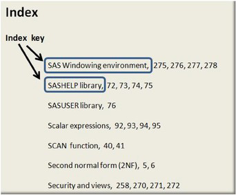
To better understand how an index works, it is useful to imagine an index located at the end of a book. A book’s index contains keywords that are listed in alphabetical order along with the corresponding page numbers displayed in ascending order, as shown in Figure 6.1. In its purest form, an index in a book is typically made available to enable readers to skip around to different pages or locations in a book. Navigating a book’s contents with an index, commonly referred to as a direct access, is contrasted with the more traditional approach of reading a book in a page-by-page sequential access manner. It is also important to recognize that for an index to retain its intrinsic value, the keyword and page number must correctly access the desired page(s) of interest at all times.

Figure 6.1: Keyword Index in Book

Indexes provide SAS users with an access method that avoids large-table scans and disk sorts, which are frequently used when the optimizer is not able to find an efficient way to service a query. An index consists of one or more columns, representing a key, to uniquely identify rows within a table. When an index is used, it finds the storage location of the rows requested by the query’s search criteria and retrieves just these rows of data.

An index is best represented as an inverted tree structure, which is sometimes referred to as a balanced tree (or b-tree), and is displayed in the following diagram. As shown in Figure 6.2, an index consists of a single root page level (starting point), zero or more intermediate levels (or nodes), and a leaf level where the actual rows of data are stored.

Figure 6.2: Inverted Tree Structure Known as a B-Tree

Because indexes are frequently too large to fit completely into primary storage (memory), they are stored on a secondary type of storage such as disk. In b-tree data structures, records or rows of data are stored in locations called leaves. B-trees are best suited to handle situations where some or part of the data resides in secondary storage. This provides an environment where the number of secondary disk accesses is reduced (fewer I/O operations), which results in a more cost-effective process.

An index typically is used to improve the speed in which subsets of data are accessed and is composed of one or more character, numeric, or mixed (alphanumeric) types of columns. Rather than sequentially accessing rows of data or physically sorting a table (as performed with an ORDER BY clause or a BY statement in PROC SORT), an index is designed to set up a logical data arrangement without the need to physically sorting it. This has a distinct advantage of reducing CPU and memory requirements, as well as reducing data access time when using WHERE clause processing.

For example, once a specific part number is known, an index can be used to look up the location of the part along with its manufacturer, cost, and availability far more efficiently than with other methods. For more information about using indexes in SAS, see The Complete Guide to Using SAS Indexes by Michael Raithel.

There is no rule that says a table has to have an index, but when an index is available it can make information access and retrieval more efficient and considerably faster.

When a query is executed in SAS software, the SQL optimizer evaluates the costs associated with the available methods and uses the most efficient method to process data. Processing can occur using a sequential table scan, or with an index if one exists. When a sequential table scan is performed, SAS starts at the beginning of the table, steps row-by-row through all of the rows in the table, and processes (retrieves) rows that match the selection criteria that is specified in the WHERE clause of the query.

Indexes should be designed to provide efficient database processing when triggered (or referenced) in a query. To better understand the impact that an index has on a database application, the following things should be kept in mind:

●         Indexes can improve the performance of queries that do not modify data because the optimizer has more choices to select from to in order to determine the fastest way to access data.

●         A table with too many indexes might actually experience a performance degradation when using INSERT, MODIFY, or DELETE operations because all indexes must be adjusted to correspond to the changes made to the data in the table.

●         A query that specifies an exact match comparison can benefit from an index. For example,

       WHERE  prodnum  =  5001;

                    < or >

       WHERE  prodtype  =  “Laptop”;

●         A query that specifies a value between a range of values can benefit from an index. For example,

       WHERE  invenqty  BETWEEN  3  AND  10;

                   < or >

       WHERE  invenqty  >= 3  AND  invenqty  <=  10;

●         Queries that produce sorted output without specifying an explicit sort operation.

●         Queries that use a LIKE comparison operator can benefit from an index when the search pattern begins with a specific character string, such as “Lap%”, but not when the search pattern begins with a wildcard, such as “%ware”.

●         Forcing the SQL optimizer to use an index in a query (with an IDXWHERE= or IDXNAME= data set option) with a small table can impede performance because SAS would traverse the index looking for matches instead of allowing the software to process data using a sequential table scan.

In the context of a database table, cardinality refers to the uniqueness, or lack thereof, of data values contained in a specific column of a table. The cardinality of a set of values refers to the uniqueness of a number of elements in a set. For example, the set CUSTNUM= {101, 201, 301, 401} contains four unique elements, and has a cardinality of four. In contrast, the set PRODTYPE = {Workstation, Laptop, Software, Software} contains four elements, three of which are unique, which results in a cardinality of three.

An understanding of the rules of cardinality and how cardinality affects a database application can help determine an optimal query plan. Table 6.1 illustrates and describes the three types of cardinality: low, normal, and high. The cardinality of a set becomes higher as the more unique elements are contained in a column. Conversely, the lower the cardinality, the more duplicate elements are contained in a column.

Table 6.1: Rules of Cardinality

An index is most effective when it is highly selective. This means that a column with high cardinality (as was presented in the previous section) is most selective when the ratio of distinct values divided by the number of rows in the table is as close to 1 as possible. The selectivity formula for an index can be quantified as follows:

$\text{Selectivity}=\frac{\text{Unique (Distinct) Rows}}{\text{Total Number Rows}}$

Note:  Perfect selectivity can only be reached on NOT NULL columns.

To determine the degree of selectivity, the number of distinct rows, and the total rows in a table for any column in a table, use the following SQL statement:

SELECT    COUNT (DISTINCT (column-name))  /  COUNT (*)  AS SELECTIVITY,

          COUNT (DISTINCT (column-name))  AS DISTINCT_VALUES,

          COUNT (*)  AS TOTAL_ROWS

    FROM  table-name;

 

<or>

 

SELECT    COUNT (DISTINCT (column-name))  /  COUNT (*)  AS SELECTIVITY

    FROM  table-name;

 

To illustrate an example of good (and in this case perfect) selectivity, the following query selects the CUSTNUM column divided by the total number of rows in the CUSTOMERS table to compute the selectivity ratio:

SQL Code

PROC SQL;

  SELECT  COUNT (DISTINCT (CUSTNUM)) / COUNT(*) AS SELECTIVITY

    FROM CUSTOMERS;

QUIT;

SAS Results

A result of 1 (18 distinct values / 18 total rows) indicates perfect selectivity and is an ideal candidate for an index because it is 100% selective of the rows in a table.

To illustrate an example of poor (and in this case bad) selectivity, the following query selects the PRODTYPE column divided by the total number of rows in the PRODUCTS table to compute the selectivity ratio:

SQL Code

PROC SQL;

  SELECT  COUNT (DISTINCT (PRODTYPE)) / COUNT(*) AS SELECTIVITY

    FROM PRODUCTS;

QUIT;

SAS Results

A result of 0.4 (4 distinct values / 10 total rows) represents low cardinality as well as less than good selectivity. Consequently, this column might not be an ideal candidate for an index because a sequential full table scan might be a more efficient way to process rows in a table.

Note:  A column’s selectivity should be recalculated from time-to-time because row inserts, updates, and deletions could change the selectivity ratio.

When defining an index, first understand the purpose the index is to serve. An important thing to remember about indexes is that they should be created only when absolutely necessary. Too many or unnecessary indexes use up computer resources and impede performance. Although the typical index takes up less space than is required by the table itself, it still represents a copy of some part of a table, and therefore requires storage space to store its contents. For this reason, care should be used when deciding when and what indexes to create.

To help determine when indexes are necessary, consider existing data as well as the way the base table(s) will be used. Acquaint yourself with queries classified as mission critical and/or essential to the success of the organization or a process. Then, determine how the data is dispersed (or the variability of the data) in the underlying base table(s) by using analytical tools such as the FREQ procedure.

If an index is used to specify some order within a table, such as manufacturer number or product number in the PRODUCTS table, you should fully assess what the impact of that index will be.

Sometimes the column(s) making up an index is obvious, and other times it is not. An index should permit the greatest flexibility so that every column in a table can be accessed and retrieved. Improvements with query results can also be achieved by assigning indexes to the most discriminating columns in a table (or columns that have many unique values), as well as to the columns that are used regularly in queries.

When an index is specified for one or more tables, a join process might actually process faster. The SQL optimizer might decide to use an index when certain conditions permit its use. Here are a few things to consider prior to creating an index:

●         If the table is small, sequential processing might be just as fast, or faster, than processing with an index.

●         If the page count, as displayed in the CONTENTS procedure, is less than three pages, then an index might serve little or no value.

●         Avoid creating more indexes than are absolutely necessary.

●         If the data subset for the index is large, then sequential access might be more efficient than using the index.

●         If the percentage of matches is approximately 15% or less (referred to as the 15% rule) of the overall population, then index usage might be beneficial.

●         The costs associated with maintaining an index can outweigh its performance value, because an index is updated each time a row in a table is added, deleted, or modified.

Two types of indexes can be defined and used in PROC SQL: simple and composite. When a simple index is created, it references only a single column. In contrast, a composite index references two or more columns in a table.

A simple index is specifically defined for one column in a table and must be the same name as the column. Suppose that you want to create an index that consists of product type (PRODTYPE) in the PRODUCTS table. Once created, the index becomes a separate object located in the SAS library.

SQL Code

PROC SQL;          ❶          ❷        ❸

  CREATE INDEX PRODTYPE ON PRODUCTS(PRODTYPE);

QUIT;

SAS Log Results

 

❶ The simple index is assigned a name of PRODTYPE, which must be the same as the column name.

❷ The simple index is defined on the PRODUCTS table.

❸ The PRODTYPE column in the PRODUCTS table is designated as the column to be used by the index.

A composite index is specifically defined for two or more columns in a table and must have a different name from the column names. Suppose that you want to create an index that consists of manufacturer number (MANUNUM) and product type (PRODTYPE) located in the PRODUCTS table. You should be aware that only one composite index is allowed per set of columns, but more than one composite index is allowed. The composite index, as with the simple index, becomes a separate object located in the SAS library.

SQL Code

PROC SQL;

  CREATE INDEX    ❶            ❷            ❸

         MANUNUM_PRODTYPE ON PRODUCTS(MANUNUM,PRODTYPE);

QUIT;

SAS Log Results

 

❶ The composite index is assigned a name of MANUNUM_PRODTYPE, which is used to represent the MANUNUM and PRODTYPE column names.

❷ The composite index is defined on the PRODUCTS table.

❸ The MANUNUM and PRODTYPE columns in the PRODUCTS table are designated as the columns to be used by the index.

The UNIQUE keyword prevents the entry of a duplicate value in an index. You should use this keyword with care because there might be times when more than one occurrence of a data value in a table is necessary. When multiple occurrences of the same value appear in a table, the UNIQUE keyword is rejected and the index is not created for that particular column.

Altering the attributes of a column that contains an associated index (simple or composite) does NOT prohibit the values in the altered column from using the index. But, if a column that contains an index is dropped, then the index is also dropped. Accordingly, when a column is dropped, any data in that index is also lost.

Readers should use caution when constructing WHERE clause expressions with the use of indexes. The SQL optimizer might prevent the use of an index and the optimization of a WHERE clause expression that contains and uses a function call. One specific function that should be avoided in a WHERE clause with index processing is the UPCASE function.

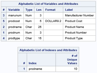
The next example shows two simple queries – the first query that specifies an UPCASE function in the WHERE clause expression and the second query that excludes the UPCASE function in the WHERE clause expression. The SAS log shows that the SQL optimizer did not optimize the first SQL query’s WHERE clause expression to use the index, but the second query did. The INFO: message showed that the simple index Prodname was selected for WHERE clause optimization. Note: To learn which, if any, of the available indexes is triggered by the WHERE clause and the SQL optimizer the MSGLEVEL=I System option is specified.

SQL Code

proc sql;

  create table work.Products as

    select *

      from mydata.Products;

  create index Prodname

    on work.Products;

quit;

 

proc contents data=work.Products;

run;

 

 

proc sql;

  select *

    from work.Products

      where UPCASE(Prodname) CONTAINS 'SOFTWARE';

 

  select *

    from work.Products

      where Prodname CONTAINS 'Software';

quit;

SAS Log Results

       proc sql;

         create table work.Products as

           select *

             from mydata.Products;

NOTE: Table WORK.PRODUCTS created, with 10 rows and 5 columns.

 

         create index Prodname

           on work.Products;

 NOTE: Simple index Prodname has been defined.

         quit;

 NOTE: PROCEDURE SQL used (Total process time):

       real time           0.01 seconds

       cpu time            0.02 seconds

       

       proc contents data=work._all_;

       run;

 

 NOTE: PROCEDURE CONTENTS used (Total process time):

       real time           0.11 seconds

       cpu time            0.11 seconds

       

 

 

       quit;

 

Results

When processing observations in a sequential manner without the use of an index, SAS reads and processes all the observations from a page of disk into memory continuing this process until the end of file. In some scenarios sequential access can be considerably costlier since the SQL optimizer will need to perform a full scan through the data.

A common assumption about an index is that as the size of the subset, based on the WHERE clause expression, becomes smaller, the index performance gains become larger. Olson (2000) describes how index processing often incurs additional computing resources. In the creation, maintenance, and usage of an index, CPU, disk space, and I/O operations will almost certainly increase so time spent understanding your query’s requirements should result in the construction of better and more efficient indexes. With index processing, SAS determines the location of the next observation using the index, and reads the observations on the page, and if necessary from a new page, satisfying the WHERE clause expression. One way to reduce the possible index processing costs is to first sort the data table in ascending order by the key column or columns and then index the table by that sorted key column or columns. As a result, performance costs using the index tend to be better since fewer reads are often performed.

When one or more indexes are no longer needed, the DROP INDEX statement can be used to remove them. Suppose that you no longer need the composite index MANUNUM_PRODTYPE (which was created earlier) because processing requirements have changed. The next example illustrates a single composite index being deleted from the SAS library.

SQL Code

PROC SQL;

  DROP INDEX MANUNUM_PRODTYPE

    FROM PRODUCTS;

QUIT;

SAS Log Results

According to the ANSI SQL standard, two or more indexes can also be deleted in a DROP INDEX statement. The next example illustrates the MANUNUM and PRODTYPE indexes being deleted from the SAS library in a single DROP INDEX statement.

SQL Code

PROC SQL;

  DROP INDEX MANUNUM, PRODTYPE

    FROM PRODUCTS;

QUIT;

SAS Log Results

Once a table is populated with data, you might need to update values in one or more of its rows. Column values in existing rows in a table can be updated with the UPDATE statement. The key to successful row updates is the creation of a well-constructed SET clause and WHERE expression. If the WHERE expression is not constructed correctly, the possibility of an update error is great.

Suppose that all laptops in the PRODUCTS table have just been discounted by 20 percent and the new price is to take effect immediately. The update would compute the discounted product cost for “Laptop” computers only. For example, the discounted price for a laptop computer would be reduced to $2,720.00 from $3,400.00.

SQL Code

PROC SQL;

  UPDATE PRODUCTS

    SET PRODCOST = PRODCOST – (PRODCOST * 0.2)

      WHERE UPCASE(PRODTYPE) = ‘LAPTOP’;

  SELECT *

    FROM PRODUCTS;

QUIT;

SAS Log Results

 

Results

1.       Data Definition Language (DDL) statements provide programmers with a way to redefine the definition of one or more existing tables (see the “Modifying Tables” section).

2.       As one or more new columns are added to a table, each is automatically added at the end of a table’s descriptor record (see the “Adding New Columns” section).

3.       To add one or more columns in a designated order, the SQL standard provides a couple of choices to choose from (see the “Controlling the Position of Columns in a Table” section).

4.       PROC SQL enables a character column (but not a numeric column) to have its length changed (see the “Changing a Column’s Length” section).

5.       A column’s format and label information can be modified with a MODIFY clause (see the “Changing a Column’s Format” and “Changing a Column’s Label” sections).

6.       The RENAME= SAS data set option must be used in a FROM clause to rename column names (see the “Renaming a Column” section).

7.       The DATASETS procedure is the recommended way to rename tables (see the “Renaming a Table” section).

8.       An index consists of one or more columns used to uniquely identify each row within a table (see the “Indexes” section).

9.       An understanding of the rules of cardinality and how it affects a database application can help determine an optimal query plan (see the “Creating a Simple Index” section).

10.      An index is most effective when it is highly selective (see the “Creating a Composite Index” section).

11.      Column values in existing rows in a table can be modified with the UPDATE statement (see the “Updating Data in a Table” section).