Chapter 3. Spanning Tree and Rapid Spanning Tree
Ethernet structure and operation are well understood because the base protocol is consistent from one version to another and the standard behaves predictably in almost every topology. Since many of the decisions regarding Ethernet—such as the network interface, signaling, and equipment type—are pre-determined, one might say that Ethernet deployments are simple and straightforward. However, proper Ethernet network operation is also dependent on adherence to topology rules and other protocols, such as the address resolution protocol. So a simple network develops some interesting, and sometimes complex, characteristics.
This chapter is about the Spanning Tree Protocol and its faster version, the Rapid Spanning Tree Protocol. These protocols wage a continuing battle to prevent against loops in Ethernet networks. A loop in an Ethernet network is created when the topology is connected back to itself. This is a problem because unlike the Internet Protocol at Layer 3, Ethernet does not have any built in protection. Therefore, it cannot prevent frames from continuously circulating. When loops occur, user connectivity can be significantly degraded if not destroyed entirely.
The Spanning Tree Protocol is active by default, and is invisible to network administrators and users alike. But because it works and is “on” by default does not necessarily mean that we can ignore it. Sometimes spanning tree is very inefficient. “On by default” also means that the protocol is working behind the scenes. Spanning tree may have taken actions making the administrator oblivious to problems on the network. This chapter will cover spanning tree usage, operation, and security concerns. The spanning tree protocol is standardized in IEEE 802.1D. While the first version of the spanning tree protocol has been replaced by rapid spanning tree, the earlier version is often the default, so understanding the earlier standard is still important. Today, spanning tree runs on most bridges and switches with the exception of some wireless equipment.
Why Are Loops Bad?
The basic problem is that at Layer 2, Ethernet does not have any ability to remove continuously circulating frames or prevent loops. Unlike IP, which has a time to live (TTL) field, Ethernet devices such as hubs and switches will simply continue to forward frames even when a loop is present. At first glance, this may not seem like such a big deal, but when you consider that a single frame passing into a switch may cause several copies to be created, the impact becomes apparent. Let’s look at a small topology. In Figure 3-1 three switches are connected in a loop.

Figure 3-1. Switching loop
When Node A communicates with Node B, the first frame sent out is an ARP request which happens to be a broadcast. Basic switch behavior is to forward this frame out all ports except for the arrival port. In this case, Switch 1 sends the frame to both Switch 2 and Switch 3. Switch 2 and Switch 3 immediately forward this broadcast frame to each other. Right after that, they send it right back to Switch 1. Switch 1 now has two copies of the frame it originally sent and to make matters worse, it does not know that they are copies. So, Switch 1 forwards these copies right back around to Switch 2 and 3. And so on, and so on... To give you an idea of how bad it can get, switches normally transmitting dozens of frames per second can be forced to transmit hundreds or even thousands of frames per second. Backplane utilization can go from less than 10% to over 80% in less than a minute. Recalling the construction of an Ethernet frame and forwarding behavior of Layer 1 and 2 devices, there is nothing to address this problem. Enter the spanning tree protocol.
Radia Perlman is the woman responsible for the Spanning Tree algorithm. The story goes that while she was working at Digital Equipment Corp (DEC), she recognized the problem and went home to think about it. She solved it on Saturday and had time to write a poem about it on Sunday. We’ll cover the protocol later but here is the poem.
Algorhyme
I think that I shall never see
A graph more lovely than a tree.
A tree whose crucial property
Is loop-free connectivity.
A tree which must be sure to span.
So packets can reach every LAN.
First the Root must be selected
By ID it is elected.
Least cost paths from Root are traced
In the tree these paths are placed.
A mesh is made by folks like me
Then bridges find a spanning tree.
The Structure of Spanning Tree BPDUs
Spanning tree requires that switches send out frames called bridge protocol data units (BPDUs) and the information contained within these BPDUs is received and processed by neighboring switches. The basic structure is shown in Figure 3-2.
There are three sections to the BPDU: protocol details, fields specific to the comparison algorithm, and the timer values. Each of these sections will be explained in greater detail later on, but to get us started, this frame is encapsulated in an 802.3 frame. Management frames such as Cisco Discovery Protocol often use 802.3 encapsulation while data frames use Ethernet Type II.

Figure 3-2. Bridge protocol data unit
The Comparison Algorithm
The whole point of spanning tree is to eliminate loops by automatically blocking ports on the network. It figures out which ports to block through the comparison algorithm. The comparison algorithm uses up to four fields to make the comparison: root identifier, root path cost, bridge identifier (transmitting bridge/switch), and the port identifier (transmitting port). From a spanning tree perspective, lower numbers are better. The order is important, with the root identifier being determined first. Figure 3-2 shows a decoded packet along with the hexadecimal version of the same packet. The spanning tree header is highlighted to show the associated hexadecimal values. Wireshark provides some clarification regarding the content of the BPDU, adding some information that is not present in the actual frame.
The information in these four fields is “compared” with information already known by the switch. The comparisons are used to make decisions regarding control of looped topologies. Spanning tree imposes a logical topology on the network by blocking ports from transmitting data frames. This means that the physical and logical topologies can differ.
Alliteration aside, the functions of the four fields follow:
- Root identifier
An eight-byte field that is a combination of the root bridge priority and the root bridge MAC address. A typical bridge priority value is 32768 (8000 in hex). The virtual local area network identifier (VLAN ID) can be added to this number. Since all of the ports on a Cisco switch start out in VLAN 1, the priority changes to 32768 + 1 (32769). The hexadecimal equivalent is 8001. In a converged or steady state topology, all BPDUs will have the same root ID. From Figure 3-2, the decoded view has a root ID of 32768/1/000af4586b80. Examining the hex section, the value 8001000af4586b80 starts after the first five bytes. This difference is the merging of the priority and VLAN id.
- Root path cost
A four-byte field describing the distance away from the root in terms of the number and speed of the links. In Figure 3-2, the path cost is 0, which means that we are looking a BPDU that came directly from the root bridge. The values for link speed are:
10BaseT
100
100BaseT
19
1000Baset
4
BPDUs leaving the root bridge will have a path cost of 0 regardless of the link speed. All other BPDUs will have topology-based values. For example, in a 100BaseT network, BPDUs that are two switches downstream would have a root path cost of 38, as shown in Figure 3-3.
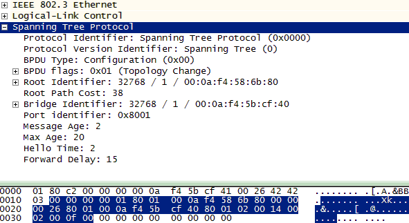
Figure 3-3. Increased path cost
- Bridge identifier
An eight-byte field that is a combination of the transmitting bridge priority and the transmitting bridge MAC address. “Transmit” is the key here because it refers to the switch sending the BPDU. Again, the typical value for the bridge priority is 32768 (8000 in hex) with an addition for any VLANs. The switch sending the current BPDU fills in its own values here. Figure 3-3 is actually a BPDU caught on the same network as the BPDU seen in Figure 3-2, just farther from the root bridge. From Figure 3-3, not only has the path cost been incremented, but the bridge ID has changed. The root ID field stays the same since all of the switches in the topology agreed on this value. The bridge ID is now 32768/1/000af45bcf40 (8001000af45bcf40 in hex) since a switch other than the root transmitted the frame. In Figure 3-2, the root ID and the bridge ID are the same, which is another indicator that the BPDU came from the root.
- Port identifier
This is the last field in the comparison algorithm. These two bytes are a combination of the transmitting port priority and the port number. A common value for the port priority is 128 (80 in hex). From Figure 3-2 we can see that the value is 8002 so the BPDU came from port 2. Figure 3-3 shows a value of 8001, which means that while the two switches were using the same port priorities, the BPDUs were sent out on different ports and, based on the different bridge ID, separate switches.
The first task of the algorithm is to elect a root bridge. It is a straightforward procedure in which the bridge with the lowest priority and MAC address combination becomes the root bridge. If all switches start with the same priority (which is common) the switch with the lowest MAC address becomes the root bridge. It does not matter which switch starts the process because switches exchange BPDUs and the spanning tree topology can change based on the information received. After the election of a root bridge, the spanning tree algorithm elects designated bridges, sets port roles, and blocks ports to eliminate loops. The following sections will first cover the building blocks of the protocol and then go through the operational aspects tying all of them together.
Some Definitions
There are several terms used within the spanning tree protocol, and understanding these will help during the topology example:
- Root bridge
This is the switch with the lowest numerical value for its priority and MAC address.
- Designated bridge
As traffic leaving a segment of the network flows to the root switch, it may pass through (be forwarded by) another switch. This switch would be the designated bridge for that segment.
- Root and designated ports
Once the topology has stabilized, all switches downstream from the root switch will have ports that are closer to the root switch and those that are farther from the root. The ports that are closer are called root ports. Ports that are farther are called designated. Another way to look at this is to say that root ports point toward the root and that traffic on its way to the root switch flows out of these ports. There is only one root port per switch. Designated ports point away from the root switch and traffic on its way to the root switch flows into these. All ports on the root switch are considered designated. Root and designated labels are called the port roles.
Spanning Tree Addressing
Spanning tree uses a specific set of addresses. In Figure 3-4, the Ethernet and Logical Link Control (LLC) headers are expanded to show the specifics. This is another view of the frame shown in Figure 3-3.
Compare the Ethernet source address in Figure 3-4 (000af45bcf41) to the bridge ID (8001000af45bcf40) seen in Figure 3-3. Removing the bridge priority leaves 000af45bcf40. Note that the Ethernet source address has simply been incremented by 1. This particular BPDU came from port 1 on the switch because of the port ID of 8001 and now this is verified by the MAC addresses because the port number is simply added to the MAC address of the switch. If this BPDU would have come from port 10, then the port ID in the spanning tree data would have been 800a and the source MAC address seen in the Ethernet frame would have been 000af45bcf4a. So the switch and its individual ports have unique MAC addresses.

Figure 3-4. BPDU addressing
Note
Occasionally you might have cause to convert a router to a bridge. In this case, the addressing does not follow this convention and the bridge ID will also vary.
The Ethernet destination MAC of 0180c2000000 is defined as the Bridge Group Address. All switches and bridges are supposed to understand and listen to this particular address. This is also why a Cisco switch can engage in spanning tree operations with a switch from another vendor. This address, along with the LLC Destination Service Access Point (DSAP) and the LLC Source Service Access Point (SSAP), are specified in IEEE 802.1D for use with the spanning tree protocol.
Port States
In an operating network, administrators are typically unaware of spanning tree port “states” because several are transitions. By the time one looks, ports that are sending/receiving traffic are already in a “forwarding” state. All ports start out in the “blocked” state. Movement between states is governed by a forwarding delay timer.
- Blocked
A port in this state can receive but not transmit BPDUs. It does not transmit or forward data frames. A port in this state may actually begin forwarding depending on the STP information received (or not received) from neighboring bridges.
- Listening
This is the first transitional state and is entered when spanning tree detects that the port may have to participate in data frame forwarding. The port will receive and process BPDUs but does not forward data frames. In this state, ports begin sending BPDUs.
- Learning
This state is similar to listening except that the port and switch now understand the topology and are preparing to forward data frames. The port will continue to receive and process BPDUs.
- Forwarding
This is the final state. A port will now forward data frames even as it continues to process any new information from incoming BPDUs.
- Shutdown/Disabled
A port that has been administratively shutdown is not participating in either forwarding of data frames or spanning tree (BPDU frames).
Spanning Tree Timers
Much of the operation of spanning tree is controlled via a series of timers. The values in use on a network can be seen in the ending BPDU data, such as in Figure 3-3 and Figure 3-7.
Hello
This timer controls the rate at which configuration BPDUs are issued from the root switch. A standard value is 2 seconds. When capturing packets this can actually get a bit annoying, as there are so many of them. The standard BPDU seen in Figure 3-4 is actually considered the “hello” message.
Max age
Switches keep track of how long they have had the current information. If the age of this information exceeds the max age timer value (20 seconds) the comparison algorithm may have to be rerun. The current age timer is reset every time new information is received via a BPDU. An example might be if the neighboring switch transmitting BPDUs was unplugged. The receiving switch would not receive anymore BPDUs and the age of the current information would start to climb. Eventually the receiver would have to find a new path to the root.
Forward delay
This timer monitors the time spent in each of the transitional port states. A 15 second limit is standard. This also provides insight into the delay between plugging in a computer and receiving a link light. The ports come up blocking, wait 15 seconds as they listen for BPDUs (listening), another 15 seconds before processing (learning) and forwarding. Therefore, a common delay for the link light is about 30 seconds.
The Operation of Spanning Tree
To better understand the operation of spanning tree, let’s run through an example using a small topology. The MAC addresses and BPDU values will be the same as those seen in the previous packets. Figure 3-5 depicts this topology. Initially all three switches are powered off. The router simply indicates a pathway off of the network but is not involved in the spanning tree decisions. The bridge priorities are all set to 32768 + VLAN or 32769 (8001 in hex) assuming VLAN 1, and the port priorities are set to 128 (80 in hex). The process begins by powering Switch 1 and then adding switches, examining the process as we go.

Figure 3-5. Small spanning tree topology
Step 1—Switch 1 Is Powered Up
When a Cisco switch is booting, all of the port link lights are amber, meaning that they are not currently forwarding traffic. In addition, when plugging a computer into a switch port, there is usually a delay before the link light goes green. This is because switch ports typically come up in the “blocking” state. The switch must first learn about the network topology before it starts forwarding traffic. This is to avoid creating an immediate loop.
Once Switch 1 has listened for and processed potential BPDU traffic, it is free to begin forwarding traffic. During this time, the ports have been transitioning between the various states. Using the debug spanning-tree events command on a Cisco switch yields the output in Figure 3-6.
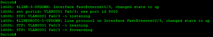
Figure 3-6. Port states
As port FastEthernet 0/3 (F0/3) comes up it transitions from blocking→listening→learning→forwarding, pausing for 15 seconds in listening and learning states.
Flowing out of ports 1 and 3 we would see the BPDUs in Figure 3-7. Note that the Ethernet source MAC addresses and the port IDs seen in the BPDU data correspond to the port transmitting the BPDU. Since Switch 1 is the only one running, it is the root switch and the transmitting switch as well. This is reflected in the BDPU root ID and bridge ID fields. The path cost for both BPDUs is 0.

Figure 3-7. Step 1 BPDUs
The result of this step can also be seen with the show spanning-tree command.
From Figure 3-8, the root ID and the bridge ID are the same. The bridge priority is listed as 32769. Port F0/1 and F0/3 are forwarding with a cost of 19 (indicating 100Mbps) and a port priority of 128. The timer values are also listed.

Figure 3-8. Step 1 show spanning tree
Step 2—Switch 2 Is Powered Up
In steady state conditions, BPDUs flow away from the root bridge. This is simply because there is no need to inform upstream switches about network conditions since the upstream switches are the original source. This is true until something in the network changes. In this case, the MAC address of Switch 2 is lower than that of Switch 1. This means that if the bridge priorities are the same (they are), Switch 2 will become the new root. The ports on Switch 2 come up blocking but listen to the BPDUs coming from Switch 1. Switch 2 notices that the value contained in the root ID field is inferior to its own bridge ID and responds with a BPDU back to Switch 1 indicating that a coup d’etat is underway. Examining the debugging output on Switch 1, we can follow its reaction.
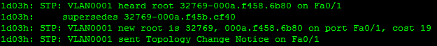
Figure 3-9. Switch 1 debug output showing a new root switch
Capturing BPDUs between Switch 1 and Switch 2 shows that the BPDUs are now flowing from Switch 2 instead of Switch 1. The important details are that the root and bridge IDs have changed. Recall that since these are the same, this BPDU came from the root. This is supported by a root path cost of 0. Compare Figure 3-10 to Figure 3-7.

Figure 3-10. BPDU from the new root
The results can also be seen in the BPDUs transmitted from Switch 1 on the other side of the topology. In Figure 3-11 the BPDU was sent from the old root (bridge ID field) but Switch 2 is advertised as the new root in the root ID field (32768/1/000af4586b80).
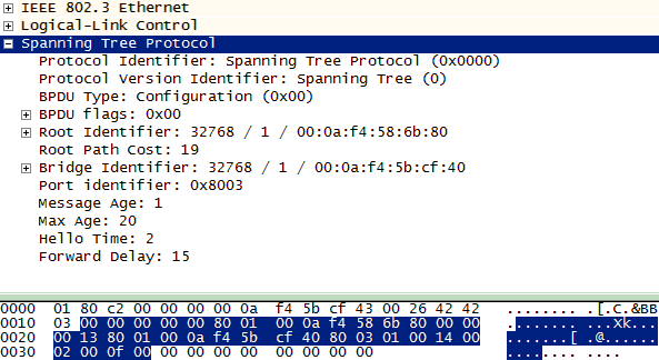
Figure 3-11. BPDU from old root advertising the new root
The path cost has also increased to 19 because traffic must now cross the 100Mbps Switch 1 in order to reach the root switch. Lastly, the summary on Switch 1 displays the changes to the topology in another form.

Figure 3-12. Switch1 show spanning tree with new root
Figure 3-9
contained the debugging results of Switch 1 receiving a BPDU from Switch
2. This event also changed the information output from the show spanning-tree command, as shown in Figure 3-12. Like most network
processes, examining the packet captures and the output from the network
devices provides a window into the operation of the protocol.
Step 3—Switch 3 Is Powered Up
With the addition of Switch 3, the topology is complete, though not yet converged. Based on MAC address and priority, all three switches will recognize Switch 2 as the root. BPDUs will flow away from Switch 2, advertising the topology information as they go. Adding Switch 3 does not change very much in the topology except to extend it. At the farthest point from Switch 2 (top computer in Figure 3-5), a capture would reveal that the path cost to the root is now 38 and that Switch 3 is the transmitting switch. This is shown in Figure 3-13.

Figure 3-13. BPDU transmitted by Switch 3
Note that the bridge ID has changed but the root ID has not. The path cost has increased to 38. The port ID is 8003.
After developing an understanding of the structure and basic operation of spanning tree, one might realize that given this small network, spanning tree is not necessary because the topology is not looped. But what if someone came along and connected Switch 2 to Switch 3 either by accident (happens all the time) or due to an interest in redundancy? That is where the fun begins. On to step 4.
Step 4—Creation of a Loop
When a physical loop is created by connecting Switches 2 and 3, spanning tree responds by blocking one of the ports in the topology. If more loops are created, more ports would be blocked until all of the loops were eliminated. Initially, the physical and logical topologies are the same. The decision as to which port is blocked is based entirely on the information used by the comparison algorithm. But we have another question to address first: How are loops detected? During normal operations, BPDUs flow away from the root. Stated another way, a switch should only receive information about the root switch from one direction. When a switch “hears” about the root via BPDUs on more than one port, a loop has occurred.
Regardless of the spanning tree version, switches react very quickly to eliminate the loop. As switches compare BPDU information, the switch with the highest values is the loser and must block a port. Figure 3-14 is a depiction of the new topology with the loop created. We know that based on the priorities and MAC addresses, Switch 2 became the root switch. Thus, all of the BPDUs seen in this network have the same value in the first field of the comparison algorithm.
Root ID – 32768/1/000af4586b80
The next field to consider is the path cost to the root. The root switch sends out a path cost of 0 from ports 2 and 3. Clearly these are the lowest path cost values and the root will not be asked to block a port. Switches 1 and 3 cannot improve upon either the root ID or the path cost. So, it is up to Switch 1 and 3 to decide which of the downstream ports will be blocked as they fire BPDUs at each other.
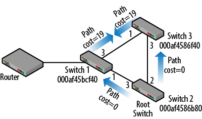
Figure 3-14. Looped topology
On the link between Switch 1 and Switch 3, BPDUs would be sent out with the same root ID and, as indicated in Figure 3-14, the same path cost. In this case, the decision as to which port to block comes down to the bridge ID. With the bridge priorities the same, the higher MAC address “loses” and Switch 1 must block a port. While the physical topology will continue as drawn in Figure 3-14, the logical topology will behave like the one seen in Figure 3-15 with port 3 on Switch 1 blocked and the loop is eliminated.

Figure 3-15. Resolved topology
The output of the show spanning
tree command run on Switch 1 (Figure 3-16) depicts the
topology changes made. Remember that the cable is still physically
connected.
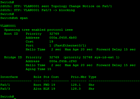
Figure 3-16. Switch 1 show spanning tree with blocked port
At the top of Figure 3-16 the event is recorded and the final state is displayed at the bottom with the interface list. Root ports, designated ports, root bridges and designated bridges were defined in a previous section. Once the topology has stabilized we can now clearly see the roles of each network device and port. In Figure 3-17, the letters B, R, and D indicate blocked, root, and designated ports, respectively.

Figure 3-17. Switch and port roles
These roles can also be seen in the output from the show spanning tree command in Figure 3-12 and Figure 3-16.
Spanning Tree Messages
In order to arrive at this new stable configuration, the switches swapped quite a bit of information via BPDUs. The spanning tree protocol has a small collection of messages, including the steady state “hello” already seen. But with the introduction of a loop and the need to block a port, it is time to talk about the other message types. The 1-byte BPDU type is set based on the message used. The 1-byte BPDU flags field provides an indication of the operation underway. The steady state values are shown in Figure 3-18. This frame was captured immediately before the loop was introduced.

Figure 3-18. BPDU type and flags
- Configuration
This is the standard message type. The BPDU type field is set to 00. The message contains all of the information discussed in this chapter. Figure 3-18 is an example of a configuration BPDU with the flags field set to 00.
- Topology Change
This BPDU is meant to indicate that a topology reconfiguration is underway. When the loop was created, Switches 1 and 3 exchanged BPDUs. Switch 3, understanding that there was a better path to the root, initiated a topology change or TC. There are a couple of events that will drive a topology change in a spanning tree topology: expiration of the max age timer, addition or removal of a switch, links going up/down, and receipt of new information via a BPDU. In the loop example, the trigger occurred when Switch 3 became aware of a second pathway to the root switch. The change to the flags field is shown in Figure 3-19.

Figure 3-19. Topology change flags
- Topology Change Notification
Upon receipt of a BPDU from Switch 3, Switch 1 now realizes that the topology is changing; BPDUs will flow in the same direction but there is a loop. Switch 1 now sends a Topology Change Notification (TCN) back to the root as shown in Figure 3-20.

Figure 3-20. Topology change notification
The TCN BPDU does not contain any configuration information. A close look at the hex for the BPDU reveals that the trailer (padding of all 0’s) is much larger to adhere to the Ethernet minimum frame size.
The topology change process continues long enough for all of the ports throughout the topology to transition to the proper state (forwarding or blocked). Per the standard, the forwarding delay timer cycles twice. So this amounts to about 30 seconds. You can actually count the number of configuration BPDUs during this time and usually come up with 15 or 16.
- Topology Change Notification Acknowledgement
When a TCN is sent (in this case from 000af45bcf41 on Switch 1), the receiving switch returns an answer in the form of a TCN ACK message as seen in Figure 3-21. This message indicates its purpose via the flags field and provides the most up-to-date information regarding the topology.

Figure 3-21. TCN acknowledgement
The last note I’d like to make regarding the flags field is that it is 1 byte in length, yet only uses a couple message types. We’ll store this little piece of information away for use later in the chapter.
Problems with Spanning Tree
Spanning tree is very good at eliminating loops. It took less than five seconds to solve the problem in our sample topology. However, when information is lost or when better pathways are created, spanning tree can be excruciatingly slow. For example, if the loop was removed from the topology by unplugging the cable between Switch 1 and 2 (reverting back to the one seen in Figure 3-5), spanning tree would not instantaneously “unblock” port 3 on Switch 1. Instead, we would have to wait for the information received by Switch 3 to age out. Switch 3 would no longer receive BPDUs from the root switch. Eventually the max age timer would expire and a topology change would begin. But how long would it take? The max age timer is 20 seconds, after which the TCN would be sent. The forwarding delay timer is 15 seconds for both the listening and learning states. So, port 3 on Switch 1 would remain blocked for 50 seconds even after the loop was gone. Any node connected to Switch 3 would be isolated for that entire time. As the network size or complexity increases, this length of time will also increase. This delay makes the original spanning tree inappropriate for a redundancy solution.
Another problem, and one of the reasons that it is good to understand the protocol, is that “automatic” spanning tree topologies can often be suboptimal in terms of forwarding. Assume that a host is connected to Switch 3 and attempts to open a web page. Based on the original blocking solution (port 3 on Switch 1), the traffic would have to flow around the entire topology as shown in Figure 3-22.
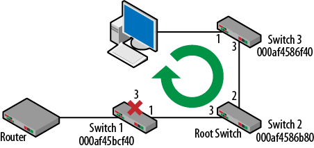
Figure 3-22. Suboptimal forwarding
In this case, the spanning tree eliminated the loop but created problems for traffic handling. In order to improve things for all nodes, the priority of Switch 1 could be changed such that it becomes the root. Recall that the bridge ID is a combination of bridge/switch priority followed by the MAC address. In Figure 3-23, the priority has been lowered to 4096 + 1 for the VLAN (1001 in hex) making Switch 1 the new root.

Figure 3-23. BPDU with priority change
The topology now resolves itself as shown in Figure 3-24. The pathway off the network for nodes connected to both Switch 2 and 3 is now straight through Switch 1. Port 3 on Switch 1 has been unblocked and port 3 on Switch 3 has been blocked.

Figure 3-24. Topology with new root based on priority
Switch to Switch: A Special Case
Regardless of topology, the whole process begins with the election of a root switch based on priority and MAC address. From there, switches with the best path cost to the root become designated bridges for the traffic traveling off of a particular network segment. In the event of a path cost tie such as that seen earlier in this chapter, the nonroot switch having the highest bridge ID (priority and MAC address) loses and must block a port. But when does the port ID field get used?
In Figure 3-25, two switches are connected directly to each other in a loop. Again, spanning tree will step in and block one of the ports. In order to determine which one, the comparison algorithm must be used:

Figure 3-25. Special case
Elect a root Switch. Assuming that the priorities are the same (32768 + 1), the deciding factor is the MAC address. Switch 1 becomes the root.
Path Cost. BPDUs flow away from the root and since both BPDUs are also leaving the root, they will have a path cost of 0.
Compare bridge IDs. Bridge ID is the ID of the transmitting bridge. In this case, both BPDUs will have the same value of 8001:000af4586b80 since they both come from the root.
Compare port IDs. This is our last chance to stop the loop. All of the other fields have had the same values in each BPDU. However, when we compare the BPDU leaving ports 1 and 2, we finally see a difference. From port 1, the port ID is 8001 (priority of 128 and a port number of 1) while the BPDU leaving port 2 on Switch 1 has a port ID of 8002 (priority of 128 and a port number of 2).
Because of the information received from Switch 1, Switch 2 now decides to block its own port 2 which terminates the loop. It is important to realize that the information contained in the BPDUs had nothing to do with Switch 2.
Cisco Improvements
Rapid spanning tree protocol (RSTP) has been part of the standards literature for more than a decade. However, it has not always been supported by vendor equipment. Even if you had equipment supporting RSTP, it might not be compatible with older bridges and switches. Cisco deployed a series of improvement to STP in an effort to help speed up convergence and port forwarding.
Portfast
Spanning tree is for bridges and switches. Hosts do not care very much about the network topology. So, when a host is connected to the network, it is not really necessary to have them wait for the transitions between the port states. In fact, devices like voice over IP phones may actually suffer because of it. This is because the phone is attempting to complete a number of transactions early in the connection process.
The command spanning-tree
portfast informs the port that it does not have to go through
the listening and learning port states. It is very handy when working in
a dynamic environment during troubleshooting or testing. However, this
is only to be used with end nodes. Accidentally connecting an interface
configured for portfast with another switch can create loops. The
potential hazards are advertised by Cisco when you issue the
command.

Figure 3-26. Portfast warning
Uplinkfast
Uplinkfast is designed to help speed up convergence in cases where an alternate path to the root switch exists. One of the downfalls of spanning tree is that it can lead to lengthy convergence delays because of the timers, even though a failover pathway might exist. Even in the small topology discussed earlier, the convergence time was 50 seconds when the loop was removed.
Using the same topology, Switches 1 and 3 will be given the
command spanning-tree uplinkfast and
become members of an uplink group with their neighbors. There are a
couple of changes to the BPDU; bridge priority and path cost are
increased. This ensures that they will not become
the root as they now have specified roles. Figure 3-27 depicts these BPDU changes.
Another look at the output from show
spanning-tree reveals that the switch has a completely
different view of the topology. The change noted in the BPDU is here but
in addition, one will be listed as an alternate. To be complete, the
blocked port was listed as alternates before (Figure 3-16) but they operated
with the longer delays.
With uplinkfast configured, when the link to the root is lost, the switch immediately fails over to the secondary pathways through Switch 3. In addition, port 3 on Switch 1 starts forwarding. This takes about 1 second as opposed to nearly a minute.
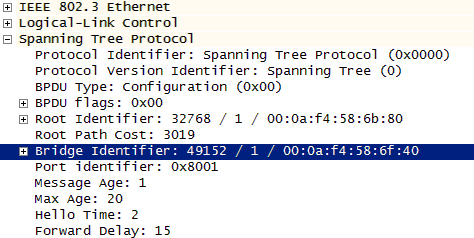
Figure 3-27. Uplinkfast BPDU

Figure 3-28. Uplinkfast output
Backbonefast
The uplinkfast goal is to improve slow convergence time for a switch that has lost its connection to the root switch. But what about when a switch elsewhere in the topology loses the connection to the root? Normally it would be “every switch for itself” and max age timers would have to be exceeded before anything could be done. For example, in topology from Figure 3-17, Switch 2 is the root and Switch 1 is blocking port 3 to eliminate the loop. Uplinkfast helped with a loss of the connection between Switch 1 and 3. But if the link between Switch 2 (root) and Switch 3 were to be lost, is there anything Switch 1 can do to help?
With backbonefast, when Switch 3 loses its connection to the root, it responds by advertising itself as the root via a BPDU sent to Switch 1. However, Switch 1 is still connected to the original root and so recognizes the BPDU from Switch 3 as inferior. Switch 1 can use a special frame called a root link query (RLQ) to determine if the root is still present. If the root still lives, Switch 1 can transition blocked port 3 immediately to the listening state without waiting for the max age timer to expire. This saves about 20 seconds in convergence time over standard spanning tree.

Figure 3-29. Root link query
Wireshark does not decode the entire root link query. Recall that this is highly proprietary and not commonly deployed. However, an examination of the data field shows us the MAC addresses of the switches involved. Even more telling is the conversation between the switches. This frame is generated from a nonroot switch upon receipt of the inferior BPDU. It is followed by an RLQ response from the root switch. Once the path to the root is established, the blocked port on Switch 1 immediately transitions to the listening state.
VLANs and Spanning Tree
Earlier in this chapter, there was an indicator that STP might be affected by VLANs. The bridge priority takes the VLAN ID into account by adding the value to 32768. From Chapter 4, VLANs are separate IP networks and exist as separate Layer 2 broadcast domains. It turns out that each VLAN can have its own instance of spanning tree running. This means that if needed, each VLAN could have a different logical topology than the other VLANs running on the same switches. In Cisco language, this is known as Per VLAN Spanning Tree, or PVST.
Consider the topology seen in Figure 3-30. On the surface, it is the exact same topology used earlier in this chapter, except that now there are VLANs running on the switches and the switches are interconnected with trunks. I’ve also added a set of servers for VLANs 4 and 5. By default, spanning tree would resolve the topology exactly as we have seen so far, even with the VLANs. This is because even with VLANs, spanning tree makes its decision the same way. While there are separate VLANs, the logical topologies will end up being the same, though they will be calculated independently.
The problem is that even on this small topology, we can see that VLAN 4 users on Switch 3 have to travel all the way around the network to access the servers. This is not true for the users on VLAN 5 since the servers are located in the center of the network. To make this more efficient, Switch 1 could be made the root for VLAN 4.
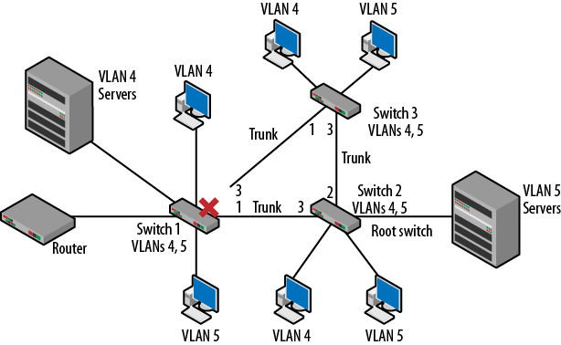
Figure 3-30. Spanning tree topology with VLANs
As before, we’ll make a small change based on priorities. In Figure 3-24, the result of
changing switch priorities is shown in the BPDU. What isn’t obvious is
that this priority change is actually for the VLAN. Specifically this was
a change for VLAN 1 since in that case, all ports were in VLAN 1. The
actual command used was spanning tree vlan 1
priority 4096. For this example, the command will be modified to
spanning tree vlan 4 priority 4096.
Note that VLAN 5 is not addressed because the root for VLAN 5 is right
where it should be. The result is that the physical topology will not
change but there will be two logical
topologies as shown in Figure 3-31.

Figure 3-31. New spanning tree topologies based on VLAN
On the left, we can see that the topology has been modified to block
port 3 on Switch 3. This modification brings the resources closer to the
VLAN 4 users. The right side topology remains the same. Examining the
show spanning tree output from earlier
in the chapter (ex. Figure 3-16 and Figure 3-28), the VLAN ID is listed as part of the
screen data. For the topologies shown in Figure 3-31, the output from the
show spanning tree command would depict the two configurations by
providing separate output for VLANs 4 and 5. It is important to realize
that packet forwarding decisions are based not just on the MAC addresses
but the VLAN IDs seen on the trunk lines as well. These details are
covered in Chapter 4.
Another important benefit to creating multiple instances of spanning tree is that for a portion of the logical traffic, ports can now be brought into service that otherwise might have blocked traffic, improving throughput and performance.
The Rapid Spanning Tree Protocol
The Spanning Tree Protocol from IEEE 802.1D is highly effective at eliminating loops but very slow at converging in other situations such as recovering pathways. Most organizations do not depend on spanning tree or other Layer 2 solutions for redundancy, load balancing or failover. Routers often replace switches where these features are desired. Cisco added improvements such as portfast, uplinkfast and backbonefast address either slow convergence or port state transitions though not all of these are in regular use.
The Rapid Spanning Tree Protocol (RSTP), which is standardized in IEEE 802.1w, improves the performance of the original spanning tree and incorporates many of the functions seen in the Cisco enhancements. In addition, it is fast enough to become a dependable component of some robust, highly reliable networks.
A couple of the significant changes include:
Switches quickly purge old information once new data is received
Several new port roles are defined.
Port states have also been modified.
In 802.1D spanning tree, once a port begins forwarding, there is no indication of the port role within the BPDU. From the BPDUs seen earlier in the chapter, we also know that while the BPDU type and flags field comprise 2 bytes of data, few values or types are used. RSTP makes use of these fields to convey additional information regarding the ports and therefore, the topology.
Rather than transitioning to forwarding and then simply becoming either a root or designated port, RSTP separates these two ideas and reduces the number of states.
| 802.1D | 802.1w |
|---|---|
Disabled | Discard |
Blocked | Discard |
Listening | Discard |
Learning | Learning |
Forwarding | Forwarding |
Blocking becomes a port role and is divided into backup and alternate blocked ports. The roles of designated and root are now variables of the port and are sent along with the BPDU. Within the flags field, the port states (learning and forwarding) and the roles are sent along with the BPDU. This is in addition to a change to the protocol version and signaling. Recall that 802.1D messages are limited to configuration, topology change notification (TCN) and the TCN ACK. RSTP adds proposals and ACKs for the proposals. An example of these changes can be seen in Figure 3-32.
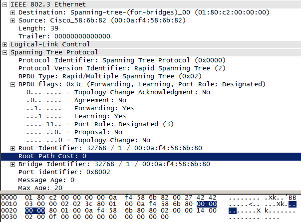
Figure 3-32. Rapid spanning tree fields
Even with these changes, much of the protocol is the same. Root ports are still those receiving BPDUs and sending TCN BPDUs (point to the root switch) and designated ports still send BPDUs and receive TCN BPDUs (point away from the root switch). Switch and port priorities are also used in similar fashion.
The Operation of RSTP
Unlike 802.1D spanning tree, in which switches only send BPDUs if they have received one from upstream, RSTP switches send BPDUs every Hello time regardless. In addition, rather than wait for the max age timer of 20 seconds to expire, RSTP only waits for three Hello times (6 seconds) before aging out neighbor information. This means that there is faster failure detection and the Hello or configuration BPDU can be thought of as a “keep alive” message. RSTP also allows immediate acceptance of inferior BPDU information in the event that the path to the root switch is lost. This is similar to the behavior of backbonefast.
Ports are now identified according to their link type without the addition of vendor improvements. Edge ports are those that do not receive BPDUs and so transition to forwarding immediately without stopping in the other port states. This is similar to portfast. An edge port receiving a BPDU converts to a standard spanning tree port. Point-to-point links are those connecting switches directly together. These ports also transition quickly to the forwarding state because a loop is less likely. This is based on the port being full duplex. These link types can also be configured manually. Figure 3-33 depicts the output of the show spanning-tree command after RSTP has been enabled. Note the changes to the link types.

Figure 3-33. RSTP show spanning tree output
On point-to-point links, switches negotiate for permission to begin forwarding via proposal and agreement. Upon changes, ports go into “sync” by blocking/discarding or converting to edge ports. The negotiation elects root ports and transitions some ports directly to forwarding. For RSTP topology changes, switches start a topology change timer for all “nonedge” designated ports and the root port. Spanning tree MAC addresses are flushed for these ports. In this way, the new information is quickly reported to the other switches in the network. Convergence time is drastically reduced making RSTP part of redundancy and failover solutions.
Alternate and backup blocked ports
Alternate ports are blocked ports that still receive BPDUs from other bridges though better pathways exist. Building on the topology used earlier, I’ve added Switch 4 downstream of Switch 3. Upon loss of the “better” pathway to the root via Switch 3, the alternate port on Switch 1 will quickly transition to forwarding. This is similar to, but much faster than the idea of uplinkfast.
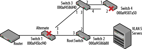
Figure 3-34. Alternate and backup ports
Backup ports receive BPDUs from their own switch but are the inferior port. In this case they are blocked but have no guarantee back to the root. This is also shown in Figure 3-34 on Switch 4. Looking closely at port 2 on Switch 4, we can understand why it was blocked. Comparing the BPDUs from Switch 3 to Switch 4, the BPDU leaving port 4 would be inferior. If port 2 on Switch 3 stopped sending BPDUs, port 4 on Switch 3 should take over. But Switch 4 is not guaranteed access to the root since the overall path did not change; it is still via Switch 3 and so is dependent upon connectivity elsewhere in the network. This is also one of the few cases where RSTP does not outperform 802.1D STP in terms of convergence.
Security
The security concerns with a protocol like spanning tree are not
usually directed at loss of data or intrusion. Instead, administrators
worry about network disruption or denial of service problems. Spanning
tree topologies are relatively easy to disrupt by injecting traffic.
Connecting to any port on a switch provides a vector for the injection.
Programs like Yersinia allow attackers to craft the necessary packets.
Attacks like this work because the switches and the protocol assume that
the incoming packets have the correct information. For example, an
attacker connecting to any one of the topologies discussed in this chapter
might inject a “bad” BPDU. The attacking BPDU might have a root priority
that is very low compared to the actual root. The “bad” BPDU causes a
topology change with all pathways resolving toward the new root. Once the
topology converges, the attacker can remove the BDPUs and force another
topology change. Changes like this also cause a network traffic to flow
toward the attacker, with the potential for exposing user data to the
attacker. Defense against this sort of attack is left to commands such as
root guard and bpdu guard, which limit the ability of attackers
to inject bad BPDUs or supplant the valid root switch. Attacks like this
can be home grown too. If a network administrator were to install a switch
without considering the spanning tree topology, the very same scenario can
occur.
Another concern for network administrators is in the wireless network. Many access points can be converted to wireless bridges. This is typically done to provide a network connection to geographically remote sites or nodes. Like an access point, a wireless bridge has both a wired and wireless interface. A little slip can result in a topology like that shown in Figure 3-35.
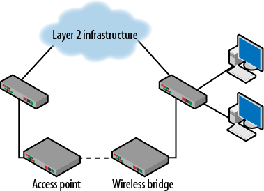
Figure 3-35. Wireless bridging loop
Depending on the type and vendor for the bridge, it may or may not participate in spanning tree. Imagine if the wireless bridge priority was lower than some of the wired switches. The topology would be forced to re-converge with the wireless bridge potentially becoming the root. Wireless bridges have nowhere near the capacity of wired switches. If the wireless bridge does not participate in spanning tree, it is possible that an unresolved loop may occur or that a port elsewhere in the topology would have to be blocked. This may limit connectivity for a section of the network.
Reading
- IEEE 802.1D bridging standard, “IEEE Standard for Local and metropolitan area networks: Media Access Control (MAC) Bridges”, (incorporates 802.1w), Jun. 2004.
- IEEE 802.1Q VLAN standard, “IEEE Standards for Local and metropolitan area networks: Virtual Bridged Local Area Networks”, (incorporates 802.1v and 802.1s), May 2006.
- RFC 5556: Transparent Interconnection of Lots of Links (TRILL): Problem and Applicability Statement
Summary
Spanning tree is a protocol that is part of almost every single Layer 2 network. Because it runs by default, it is often misunderstood or ignored entirely. However, spanning tree, and the faster rapid spanning tree, may serve a critical role in the network in protecting the Ethernet network from Layer 2 loops. The scenarios and packets described in this chapter depict the operation and expected behavior of this ubiquitous process. Rapid and 802.1D spanning have many of the same behaviors, but because of improvements to convergence speed, rapid spanning tree is the better choice for redundancy in networks. Though the protocols have been around for awhile, and some of the functions have been supplanted by routers, work continues in the area of Layer 2 loop resolution. Projects like TRILL (Transparent Interconnection of Lots of Links) indicate that folks, especially Radia Perlman, are not done thinking about the problem.
Review Questions
Spanning tree is defined in what standard?
The main purpose of spanning tree is to eliminate logical loops.
TRUE
FALSE
What are the four fields used in the comparison algorithm?
What are the components of the root ID field?
What is the destination MAC address used on a BPDU?
Describe the difference between a root port and a designated port.
What are the values for the hello, max age and hello timers?
Name three Cisco improvements to spanning tree.
Rapid Spanning Tree is appropriate for maintaining high speed redundancy in networks.
TRUE
FALSE
Rapid spanning tree defined what two types of blocked ports?
Review Answers
802.1D
TRUE
Root ID, path cost, bridge ID, port ID
Bridge priority and MAC address
01:80:c2:00:00:00
Root ports point to the root switch and designated ports point away. Traffic flows into designated ports on its way to the root switch and out of root ports.
15, 20 and 2 seconds
Portfast, uplinkfast and backbonefast
TRUE
Alternate and backup
Lab Activities
Activity 1—Capture of a BPDU
Materials: A computer with an active network connection to a switch and packet capture software (Wireshark)
If not already connected to the switch, connected the computer NIC to the switch.
Once the link light turns green, start the packet capture software.
Examine the packets captured and find a BPDU.
Open the BPDU and analyze the fields used by the comparison algorithm. What are the values?
Activity 2—BPDU Address Analysis
Materials: A computer with an active network connection to a switch and packet capture software (Wireshark)
Using the BPDU captured in Activity 1, examine the addressing used. Look for the following:
Source and destination MAC addresses
Root bridge MAC address
Transmit Bridge MAC address.
How are these related to each other? How are they used?
Activity 3—Looping the Switch Back to Itself
Materials: Managed Switch
Prior to starting this activity, determine what you are going to do and try to determine what will happen with this loop.
Using an Ethernet cable, loop one port on the switch to another.
What happens to the link lights?
In the management interface, what is the status of the ports? Are any blocked? If so, which one and why? Be very specific in your answer.
Activity 4—Looping Switches Together
Materials: Two or three managed switches, a computer capable of capturing packets
This activity assumes access to a collection of switches. Two will be sufficient for the experiments.
As in Activity 3, try to determine what will happen when the loop is created. Be very specific about what will happen and why.
Connect the 2 or 3 switches in a line. Which switch is the root? What will the BPDU look like at a point farthest from the root? Consider the four fields of the comparison algorithm.
Connect the switches in a loop. What port will be blocked? Why? What will the changes be to the BPDUs on each segment of the network?
Activity 5—Removing the Loop
Materials: Two or three managed switches, a computer capable of capturing packets
Using the topology from Activity 4, remove the physical loop you created.
How long does it take for the blocked port to move to the forwarding state?
What happens if you change the switch priorities on one of the nonroot switches? How long does it take for the effect to be reflected in the network topology and BPDUs?