11
Combining Pandas Objects
Introduction
A wide variety of options are available to combine two or more DataFrames or Series together. The append method is the least flexible and only allows for new rows to be appended to a DataFrame. The concat method is very versatile and can combine any number of DataFrames or Series on either axis. The join method provides fast lookups by aligning a column of one DataFrame to the index of others. The merge method provides SQL-like capabilities to join two DataFrames together.
Appending new rows to DataFrames
When performing data analysis, it is far more common to create new columns than new rows. This is because a new row of data usually represents a new observation, and as an analyst, it is typically not your job to continually capture new data. Data capture is usually left to other platforms like relational database management systems. Nevertheless, it is a necessary feature to know as it will crop up from time to time.
In this recipe, we will begin by appending rows to a small dataset with the .loc attribute and then transition to using the .append method.
How to do it…
- Read in the
namesdataset, and output it:>>> import pandas as pd >>> import numpy as np >>> names = pd.read_csv('data/names.csv') >>> names Name Age 0 Cornelia 70 1 Abbas 69 2 Penelope 4 3 Niko 2 - Let's create a list that contains some new data and use the
.locattribute to set a single row label equal to this new data:>>> new_data_list = ['Aria', 1] >>> names.loc[4] = new_data_list >>> names Name Age 0 Cornelia 70 1 Abbas 69 2 Penelope 4 3 Niko 2 4 Aria 1 - The
.locattribute uses labels to refer to the rows. In this case, the row labels exactly match the integer location. It is possible to append more rows with non-integer labels:>>> names.loc['five'] = ['Zach', 3] >>> names Name Age 0 Cornelia 70 1 Abbas 69 2 Penelope 4 3 Niko 2 4 Aria 1 five Zach 3 - To be more explicit in associating variables to values, you may use a dictionary. Also, in this step, we can dynamically choose the new index label to be the length of the DataFrame:
>>> names.loc[len(names)] = {'Name':'Zayd', 'Age':2} >>> names Name Age 0 Cornelia 70 1 Abbas 69 2 Penelope 4 3 Niko 2 4 Aria 1 five Zach 3 6 Zayd 2 - A Series can hold the new data as well and works exactly the same as a dictionary:
>>> names.loc[len(names)] = pd.Series({'Age':32, 'Name':'Dean'}) >>> names Name Age 0 Cornelia 70 1 Abbas 69 2 Penelope 4 3 Niko 2 4 Aria 1 five Zach 3 6 Zayd 2 7 Dean 32 - The preceding operations all use the
.locattribute to make changes to thenamesDataFrame in-place. There is no separate copy of the DataFrame that is returned. In the next few steps, we will look at the.appendmethod, which does not modify the calling DataFrame. Instead, it returns a new copy of the DataFrame with the appended row(s). Let's begin with the originalnamesDataFrame and attempt to append a row. The first argument to.appendmust be either another DataFrame, Series, dictionary, or a list of these, but not a list like the one in step 2. Let's see what happens when we attempt to use a dictionary with.append:>>> names = pd.read_csv('data/names.csv') >>> names.append({'Name':'Aria', 'Age':1}) Traceback (most recent call last): ... TypeError: Can only append a Series if ignore_index=True or if the Series has a name - This error message appears to be slightly incorrect. We are passing a dictionary and not a Series but nevertheless, it gives us instructions on how to correct it, we need to pass the
ignore_index=Trueparameter:>>> names.append({'Name':'Aria', 'Age':1}, ignore_index=True) Name Age 0 Cornelia 70 1 Abbas 69 2 Penelope 4 3 Niko 2 4 Aria 1 - This works but
ignore_indexis a sneaky parameter. When set toTrue, the old index will be removed completely and replaced with aRangeIndexfrom 0 to n-1. For instance, let's specify an index for thenamesDataFrame:>>> names.index = ['Canada', 'Canada', 'USA', 'USA'] >>> names Name Age Canada Cornelia 70 Canada Abbas 69 USA Penelope 4 USA Niko 2 - Rerun the code from step 7, and you will get the same result. The original index is completely ignored.
- Let's continue with this names DataFrame with the country strings in the index. Let's append a Series that has a
nameattribute with the.appendmethod:>>> s = pd.Series({'Name': 'Zach', 'Age': 3}, name=len(names)) >>> s Name Zach Age 3 Name: 4, dtype: object >>> names.append(s) Name Age Canada Cornelia 70 Canada Abbas 69 USA Penelope 4 USA Niko 2 4 Zach 3 - The
.appendmethod is more flexible than the.locattribute. It supports appending multiple rows at the same time. One way to accomplish this is by passing in a list of Series:>>> s1 = pd.Series({'Name': 'Zach', 'Age': 3}, name=len(names)) >>> s2 = pd.Series({'Name': 'Zayd', 'Age': 2}, name='USA') >>> names.append([s1, s2]) Name Age Canada Cornelia 70 Canada Abbas 69 USA Penelope 4 USA Niko 2 4 Zach 3 USA Zayd 2 - Small DataFrames with only two columns are simple enough to manually write out all the column names and values. When they get larger, this process will be quite painful. For instance, let's take a look at the 2016 baseball dataset:
>>> bball_16 = pd.read_csv('data/baseball16.csv') >>> bball_16 playerID yearID stint teamID ... HBP SH SF GIDP 0 altuv... 2016 1 HOU ... 7.0 3.0 7.0 15.0 1 bregm... 2016 1 HOU ... 0.0 0.0 1.0 1.0 2 castr... 2016 1 HOU ... 1.0 1.0 0.0 9.0 3 corre... 2016 1 HOU ... 5.0 0.0 3.0 12.0 4 gatti... 2016 1 HOU ... 4.0 0.0 5.0 12.0 .. ... ... ... ... ... ... ... ... ... 11 reedaj01 2016 1 HOU ... 0.0 0.0 1.0 1.0 12 sprin... 2016 1 HOU ... 11.0 0.0 1.0 12.0 13 tucke... 2016 1 HOU ... 2.0 0.0 0.0 2.0 14 valbu... 2016 1 HOU ... 1.0 3.0 2.0 5.0 15 white... 2016 1 HOU ... 2.0 0.0 2.0 6.0 - This dataset contains 22 columns and it would be easy to mistype a column name or forget one altogether if you were manually entering new rows of data. To help protect against these mistakes, let's select a single row as a Series and chain the
.to_dictmethod to it to get an example row as a dictionary:>>> data_dict = bball_16.iloc[0].to_dict() >>> data_dict {'playerID': 'altuvjo01', 'yearID': 2016, 'stint': 1, 'teamID': 'HOU', 'lgID': 'AL', 'G': 161, 'AB': 640, 'R': 108, 'H': 216, '2B': 42, '3B': 5, 'HR': 24, 'RBI': 96.0, 'SB': 30.0, 'CS': 10.0, 'BB': 60, 'SO': 70.0, 'IBB': 11.0, 'HBP': 7.0, 'SH': 3.0, 'SF': 7.0, 'GIDP': 15.0} - Clear the old values with a dictionary comprehension assigning any previous string value as an empty string and all others as missing values. This dictionary can now serve as a template for any new data you would like to enter:
>>> new_data_dict = {k: '' if isinstance(v, str) else ...     np.nan for k, v in data_dict.items()}
>>> new_data_dict
{'playerID': '', 'yearID': nan, 'stint': nan, 'teamID': '', 'lgID': '', 'G': nan, 'AB': nan, 'R': nan, 'H': nan, '2B': nan, '3B': nan, 'HR': nan, 'RBI': nan, 'SB': nan, 'CS': nan, 'BB': nan, 'SO': nan, 'IBB': nan, 'HBP': nan, 'SH': nan, 'SF': nan, 'GIDP': nan}
How it works…
The .loc attribute is used to select and assign data based on the row and column labels. The first value passed to it represents the row label. In step 2, names.loc[4] refers to the row with a label equal to the integer 4. This label does not currently exist in the DataFrame. The assignment statement creates a new row with data provided by the list. As was mentioned in the recipe, this operation modifies the names DataFrame itself. If there were a previously existing row with a label equal to the integer 4, this command would have written over it. Using in-place modification makes this indexing operator riskier to use than the .append method, which never modifies the original calling DataFrame. Throughout this book we have advocated chaining operations, and you should follow suit.
Any valid label may be used with the .loc attribute, as seen in step 3. Regardless of what the new label value is, the new row is always appended to the end. Even though assigning with a list works, for clarity, it is best to use a dictionary so that we know exactly which columns are associated with each value, as done in step 4.
Steps 4 and 5 show a trick to dynamically set the new label to be the current number of rows in the DataFrame. Data stored in a Series will also get assigned correctly as long as the index labels match the column names.
The rest of the steps use the .append method, which is a method that only appends new rows to DataFrames. Most DataFrame methods allow both row and column manipulation through an axis parameter. One exception is the .append method, which can only append rows to DataFrames.
Using a dictionary of column names mapped to values isn't enough information for .append to work, as seen by the error message in step 6. To correctly append a dictionary without a row name, you will have to set the .ignore_index parameter to True.
Step 10 shows you how to keep the old index by converting your dictionary to a Series. Make sure to use the name parameter, which is then used as the new index label. Any number of rows may be added with append in this manner by passing a list of Series as the first argument.
When wanting to append rows in this manner with a much larger DataFrame, you can avoid lots of typing and mistakes by converting a single row to a dictionary with the .to_dict method and then using a dictionary comprehension to clear out all the old values replacing them with some defaults. This can serve as a template for new rows.
There's more…
Appending a single row to a DataFrame is a fairly expensive operation and if you find yourself writing a loop to append single rows of data to a DataFrame, then you are doing it wrong. Let's first create 1,000 rows of new data as a list of Series:
>>> random_data = []
>>> for i in range(1000):
...     d = dict()
...     for k, v in data_dict.items():
...         if isinstance(v, str):
...             d[k] = np.random.choice(list('abcde'))
...         else:
...             d[k] = np.random.randint(10)
...     random_data.append(pd.Series(d, name=i + len(bball_16)))
>>> random_data[0]
2B    3
3B    9
AB    3
BB    9
CS    4
Name: 16, dtype: object
Let's time how long it takes to loop through each item making one append at a time:
>>> %%timeit
>>> bball_16_copy = bball_16.copy()
>>> for row in random_data:
...     bball_16_copy = bball_16_copy.append(row)
4.88 s ± 190 ms per loop (mean ± std. dev. of 7 runs, 1 loop each)
That took nearly five seconds for only 1,000 rows. If we instead pass in the entire list of Series, we get an enormous speed increase:
>>> %%timeit
>>> bball_16_copy = bball_16.copy()
>>> bball_16_copy = bball_16_copy.append(random_data)
78.4 ms ± 6.2 ms per loop (mean ± std. dev. of 7 runs, 10 loops each)
If you pass in a list of Series objects, the time has been reduced to under one-tenth of a second. Internally, pandas converts the list of Series to a single DataFrame and then appends the data.
Concatenating multiple DataFrames together
The concat function enables concatenating two or more DataFrames (or Series) together, both vertically and horizontally. As per usual, when dealing with multiple pandas objects simultaneously, concatenation doesn't happen haphazardly but aligns each object by their index.
In this recipe, we combine DataFrames both horizontally and vertically with the concat function and then change the parameter values to yield different results.
How to do it…
- Read in the 2016 and 2017 stock datasets, and make their ticker symbol the index:
>>> stocks_2016 = pd.read_csv('data/stocks_2016.csv', ... index_col='Symbol') >>> stocks_2017 = pd.read_csv('data/stocks_2017.csv', ... index_col='Symbol') >>> stocks_2016 Shares Low High Symbol AAPL 80 95 110 TSLA 50 80 130 WMT 40 55 70 >>> stocks_2017 Shares Low High Symbol AAPL 50 120 140 GE 100 30 40 IBM 87 75 95 SLB 20 55 85 TXN 500 15 23 TSLA 100 100 300 - Place all the stock datasets into a single list, and then call the
concatfunction to concatenate them together along the default axis (0):>>> s_list = [stocks_2016, stocks_2017] >>> pd.concat(s_list) Shares Low High Symbol AAPL 80 95 110 TSLA 50 80 130 WMT 40 55 70 AAPL 50 120 140 GE 100 30 40 IBM 87 75 95 SLB 20 55 85 TXN 500 15 23 TSLA 100 100 300 - By default, the
concatfunction concatenates DataFrames vertically, one on top of the other. One issue with the preceding DataFrame is that there is no way to identify the year of each row. Theconcatfunction allows each piece of the resulting DataFrame to be labeled with thekeysparameter. This label will appear in the outermost index level of the concatenated frame and force the creation of aMultiIndex. Also, thenamesparameter has the ability to rename each index level for clarity:>>> pd.concat(s_list, keys=['2016', '2017'], ... names=['Year', 'Symbol']) Shares Low High Year Symbol 2016 AAPL 80 95 110 TSLA 50 80 130 WMT 40 55 70 2017 AAPL 50 120 140 GE 100 30 40 IBM 87 75 95 SLB 20 55 85 TXN 500 15 23 TSLA 100 100 300 - It is also possible to concatenate horizontally by changing the
axisparameter tocolumnsor1:>>> pd.concat(s_list, keys=['2016', '2017'], ... axis='columns', names=['Year', None]) Year 2016 2017 Shares Low High Shares Low High AAPL 80.0 95.0 110.0 50.0 120.0 140.0 GE NaN NaN NaN 100.0 30.0 40.0 IBM NaN NaN NaN 87.0 75.0 95.0 SLB NaN NaN NaN 20.0 55.0 85.0 TSLA 50.0 80.0 130.0 100.0 100.0 300.0 TXN NaN NaN NaN 500.0 15.0 23.0 WMT 40.0 55.0 70.0 NaN NaN NaN - Notice that missing values appear whenever a stock symbol is present in one year but not the other. The
concatfunction, by default, uses an outer join, keeping all rows from each DataFrame in the list. However, it gives us an option to keep only rows that have the same index values in both DataFrames. This is referred to as an inner join. We set thejoinparameter toinnerto change the behavior:>>> pd.concat(s_list, join='inner', keys=['2016', '2017'], ... axis='columns', names=['Year', None]) Year 2016 2017 Shares Low High Shares Low High Symbol AAPL 80 95 110 50 120 140 TSLA 50 80 130 100 100 300
How it works…
The concat function accepts a list as the first parameter. This list must be a sequence of pandas objects, typically a list of DataFrames or Series. By default, all these objects will be stacked vertically, one on top of the other. In this recipe, only two DataFrames are concatenated, but any number of pandas objects work. When we were concatenating vertically, the DataFrames align by their column names.
In this dataset, all the column names were the same so each column in the 2017 data lined up precisely under the same column name in the 2016 data. However, when they were concatenated horizontally, as in step 4, only two of the index labels matched from both years – AAPL and TSLA. Therefore, these ticker symbols had no missing values for either year. There are two types of alignment possible using concat, outer (the default), and inner referred to by the join parameter.
There's more…
The .append method is a heavily watered-down version of concat that can only append new rows to a DataFrame. Internally, .append just calls the concat function. For instance, step 2 from this recipe may be duplicated with the following:
>>> stocks_2016.append(stocks_2017)
Shares  Low  High
Symbol
AAPL        80   95   110
TSLA        50   80   130
WMT         40   55    70
AAPL        50  120   140
GE         100   30    40
IBM         87   75    95
SLB         20   55    85
TXN        500   15    23
TSLA       100  100   300
Understanding the differences between concat, join, and merge
The .merge and .join DataFrame (and not Series) methods and the concat function all provide very similar functionality to combine multiple pandas objects together. As they are so similar and they can replicate each other in certain situations, it can get very confusing regarding when and how to use them correctly.
To help clarify their differences, take a look at the following outline:
concat:
- A pandas function
- Combines two or more pandas objects vertically or horizontally
- Aligns only on the index
- Errors whenever a duplicate appears in the index
- Defaults to outer join with the option for inner join
.join:
- A DataFrame method
- Combines two or more pandas objects horizontally
- Aligns the calling DataFrame's column(s) or index with the other object's index (and not the columns)
- Handles duplicate values on the joining columns/index by performing a Cartesian product
- Defaults to left join with options for inner, outer, and right
.merge:
- A DataFrame method
- Combines exactly two DataFrames horizontally
- Aligns the calling DataFrame's column(s) or index with the other DataFrame's column(s) or index
- Handles duplicate values on the joining columns or index by performing a cartesian product
- Defaults to inner join with options for left, outer, and right
In this recipe, we will combine DataFrames. The first situation is simpler with concat while the second is simpler with .merge.
How to do it…
- Let's read in stock data for 2016, 2017, and 2018 into a list of DataFrames using a loop instead of three different calls to the
read_csvfunction:>>> years = 2016, 2017, 2018 >>> stock_tables = [pd.read_csv( ... f'data/stocks_{year}.csv', index_col='Symbol') ... for year in years] >>> stocks_2016, stocks_2017, stocks_2018 = stock_tables >>> stocks_2016 Shares Low High Symbol AAPL 80 95 110 TSLA 50 80 130 WMT 40 55 70 >>> stocks_2017 Shares Low High Symbol AAPL 50 120 140 GE 100 30 40 IBM 87 75 95 SLB 20 55 85 TXN 500 15 23 TSLA 100 100 300 >>> stocks_2018 Shares Low High Symbol AAPL 40 135 170 AMZN 8 900 1125 TSLA 50 220 400 - The
concatfunction is the only pandas method that is able to combine DataFrames vertically. Let's do this by passing it the liststock_tables:>>> pd.concat(stock_tables, keys=[2016, 2017, 2018]) Shares Low High Symbol 2016 AAPL 80 95 110 TSLA 50 80 130 WMT 40 55 70 2017 AAPL 50 120 140 GE 100 30 40 ... ... ... ... TXN 500 15 23 TSLA 100 100 300 2018 AAPL 40 135 170 AMZN 8 900 1125 TSLA 50 220 400 - It can also combine DataFrames horizontally by changing the
axisparameter tocolumns:>>> pd.concat(dict(zip(years, stock_tables)), axis='columns') 2016 ... 2018 Shares Low High ... Shares Low High AAPL 80.0 95.0 110.0 ... 40.0 135.0 170.0 AMZN NaN NaN NaN ... 8.0 900.0 1125.0 GE NaN NaN NaN ... NaN NaN NaN IBM NaN NaN NaN ... NaN NaN NaN SLB NaN NaN NaN ... NaN NaN NaN TSLA 50.0 80.0 130.0 ... 50.0 220.0 400.0 TXN NaN NaN NaN ... NaN NaN NaN WMT 40.0 55.0 70.0 ... NaN NaN NaN - Now that we have started combining DataFrames horizontally, we can use the
.joinand.mergemethods to replicate this functionality ofconcat. Here, we use the.joinmethod to combine thestock_2016andstock_2017DataFrames. By default, the DataFrames align on their index. If any of the columns have the same names, then you must supply a value to thelsuffixorrsuffixparameters to distinguish them in the result:>>> stocks_2016.join(stocks_2017, lsuffix='_2016', ... rsuffix='_2017', how='outer') Shares_2016 Low_2016 ... Low_2017 High_2017 Symbol ... AAPL 80.0 95.0 ... 120.0 140.0 GE NaN NaN ... 30.0 40.0 IBM NaN NaN ... 75.0 95.0 SLB NaN NaN ... 55.0 85.0 TSLA 50.0 80.0 ... 100.0 300.0 TXN NaN NaN ... 15.0 23.0 WMT 40.0 55.0 ... NaN NaN - To replicate the output of the
concatfunction from step 3, we can pass a list of DataFrames to the.joinmethod:>>> other = [stocks_2017.add_suffix('_2017'), ... stocks_2018.add_suffix('_2018')] >>> stocks_2016.add_suffix('_2016').join(other, how='outer') Shares_2016 Low_2016 ... Low_2018 High_2018 AAPL 80.0 95.0 ... 135.0 170.0 TSLA 50.0 80.0 ... 220.0 400.0 WMT 40.0 55.0 ... NaN NaN GE NaN NaN ... NaN NaN IBM NaN NaN ... NaN NaN SLB NaN NaN ... NaN NaN TXN NaN NaN ... NaN NaN AMZN NaN NaN ... 900.0 1125.0 - Let's check whether they are equal:
>>> stock_join = stocks_2016.add_suffix('_2016').join(other, ... how='outer') >>> stock_concat = ( ... pd.concat( ... dict(zip(years, stock_tables)), axis="columns") ... .swaplevel(axis=1) ... .pipe(lambda df_: ... df_.set_axis(df_.columns.to_flat_index(), axis=1)) ... .rename(lambda label: ... "_".join([str(x) for x in label]), axis=1) ... ) >>> stock_join.equals(stock_concat) True - Now, let's turn to the
.mergemethod that, unlikeconcatand.join, can only combine two DataFrames together. By default,.mergeattempts to align the values in the columns that have the same name for each of the DataFrames. However, you can choose to have it align on the index by setting the Boolean parametersleft_indexandright_indextoTrue. Let's merge the 2016 and 2017 stock data together:>>> stocks_2016.merge(stocks_2017, left_index=True, ... right_index=True) Shares_x Low_x High_x Shares_y Low_y High_y Symbol AAPL 80 95 110 50 120 140 TSLA 50 80 130 100 100 300 - By default,
.mergeuses an inner join and automatically supplies suffixes for identically named columns. Let's change to an outer join and then perform another outer join of the 2018 data to replicate the behavior ofconcat. Note that in pandas 1.0, themergeindex will be sorted and theconcatversion won't be:>>> stock_merge = (stocks_2016 ... .merge(stocks_2017, left_index=True, ... right_index=True, how='outer', ... suffixes=('_2016', '_2017')) ... .merge(stocks_2018.add_suffix('_2018'), ... left_index=True, right_index=True, ... how='outer') ... ) >>> stock_concat.sort_index().equals(stock_merge) True - Now let's turn our comparison to datasets where we are interested in aligning together the values of columns and not the index or column labels themselves. The
.mergemethod is built for this situation. Let's take a look at two new small datasets,food_pricesandfood_transactions:>>> names = ['prices', 'transactions'] >>> food_tables = [pd.read_csv('data/food_{}.csv'.format(name)) ... for name in names] >>> food_prices, food_transactions = food_tables >>> food_prices item store price Date 0 pear A 0.99 2017 1 pear B 1.99 2017 2 peach A 2.99 2017 3 peach B 3.49 2017 4 banana A 0.39 2017 5 banana B 0.49 2017 6 steak A 5.99 2017 7 steak B 6.99 2017 8 steak B 4.99 2015 >>> food_transactions custid item store quantity 0 1 pear A 5 1 1 banana A 10 2 2 steak B 3 3 2 pear B 1 4 2 peach B 2 5 2 steak B 1 6 2 coconut B 4 - If we wanted to find the total amount of each transaction, we would need to join these tables on the
itemandstorecolumns:>>> food_transactions.merge(food_prices, on=['item', 'store']) custid item store quantity price Date 0 1 pear A 5 0.99 2017 1 1 banana A 10 0.39 2017 2 2 steak B 3 6.99 2017 3 2 steak B 3 4.99 2015 4 2 steak B 1 6.99 2017 5 2 steak B 1 4.99 2015 6 2 pear B 1 1.99 2017 7 2 peach B 2 3.49 2017 - The price is now aligned correctly with its corresponding item and store, but there is a problem. Customer 2 has a total of four
steakitems. As thesteakitem appears twice in each table for storeB, a Cartesian product takes place between them, resulting in four rows. Also, notice that the item,coconut, is missing because there was no corresponding price for it. Let's fix both of these issues:>>> food_transactions.merge(food_prices.query('Date == 2017'), ... how='left') custid item store quantity price Date 0 1 pear A 5 0.99 2017.0 1 1 banana A 10 0.39 2017.0 2 2 steak B 3 6.99 2017.0 3 2 pear B 1 1.99 2017.0 4 2 peach B 2 3.49 2017.0 5 2 steak B 1 6.99 2017.0 6 2 coconut B 4 NaN NaN - We can replicate this with the
.joinmethod, but we must first put the joining columns of thefood_pricesDataFrame into the index:>>> food_prices_join = food_prices.query('Date == 2017') ... .set_index(['item', 'store']) >>> food_prices_join price Date item store pear A 0.99 2017 B 1.99 2017 peach A 2.99 2017 B 3.49 2017 banana A 0.39 2017 B 0.49 2017 steak A 5.99 2017 B 6.99 2017 - The
.joinmethod only aligns with the index of the passed DataFrame but can use the index or the columns of the calling DataFrame. To use columns for alignment on the calling DataFrame, you will need to pass them to theonparameter:>>> food_transactions.join(food_prices_join, on=['item', 'store']) custid item store quantity price Date 0 1 pear A 5 0.99 2017.0 1 1 banana A 10 0.39 2017.0 2 2 steak B 3 6.99 2017.0 3 2 pear B 1 1.99 2017.0 4 2 peach B 2 3.49 2017.0 5 2 steak B 1 6.99 2017.0 6 2 coconut B 4 NaN NaNThe output matches the result from step 11. To replicate this with the
concatfunction, you would need to put theitemandstorecolumns into the index of both DataFrames. However, in this particular case, an error would be produced as a duplicate index value occurs in at least one of the DataFrames (with itemsteakand storeB):>>> pd.concat([food_transactions.set_index(['item', 'store']), ... food_prices.set_index(['item', 'store'])], ... axis='columns') Traceback (most recent call last): ... ValueError: cannot handle a non-unique multi-index!
How it works…
It can be tedious to repeatedly write the read_csv function when importing many DataFrames at the same time. One way to automate this process is to put all the filenames in a list and iterate through them with a for loop. This was done in step 1 with a list comprehension.
At the end of step 1, we unpack the list of DataFrames into their own appropriately named variables so that each table may be easily and clearly referenced. The nice thing about having a list of DataFrames is that it is the exact requirement for the concat function, as seen in step 2. Notice how step 2 uses the keys parameter to name each chunk of data. This can be also be accomplished by passing a dictionary to concat, as done in step 3.
In step 4, we must change the type of .join to outer to include all of the rows in the passed DataFrame that do not have an index present in the calling DataFrame. In step 5, the passed list of DataFrames cannot have any columns in common. Although there is an rsuffix parameter, it only works when passing a single DataFrame and not a list of them. To work around this limitation, we change the names of the columns beforehand with the .add_suffix method, and then call the .join method.
In step 7, we use .merge, which defaults to aligning on all column names that are the same in both DataFrames. To change this default behavior, and align on the index of either one or both, set the left_index or right_index parameters to True. Step 8 finishes the replication with two calls to .merge. As you can see, when you are aligning multiple DataFrames on their index, concat is usually going to be a far better choice than .merge.
In step 9, we switch gears to focus on a situation where the .merge method has the advantage. The .merge method is the only one capable of aligning both the calling and passed DataFrame by column values. Step 10 shows you how easy it is to merge two DataFrames. The on parameter is not necessary but provided for clarity.
Unfortunately, it is very easy to duplicate or drop data when combining DataFrames, as shown in step 10. It is vital to take some time to do some sanity checks after combining data. In this instance, the food_prices dataset had a duplicate price for steak in store B, so we eliminated this row by querying for only the current year in step 11. We also change to a left join to ensure that each transaction is kept regardless if a price is present or not.
It is possible to use .join in these instances, but all the columns in the passed DataFrame must be moved into the index first. Finally, concat is going to be a poor choice whenever you intend to align data by values in their columns.
In summary, I find myself using .merge unless I know that the indexes align.
There's more…
It is possible to read all files from a particular directory into DataFrames without knowing their names. Python provides a few ways to iterate through directories, with the glob module being a popular choice. The gas prices directory contains five different CSV files, each having weekly prices of a particular grade of gas beginning from 2007. Each file has just two columns – the date for the week and the price. This is a perfect situation to iterate through all the files, read them into DataFrames, and combine them all together with the concat function.
The glob module has the glob function, which takes a single parameter – the location of the directory you would like to iterate through as a string. To get all the files in the directory, use the string *. In this example, ''*.csv' returns only files that end in .csv. The result from the glob function is a list of string filenames, which can be passed to the read_csv function:
>>> import glob
>>> df_list = []
>>> for filename in glob.glob('data/gas prices *.csv'):
...     df_list.append(pd.read_csv(filename, index_col='Week',
...     parse_dates=['Week']))
>>> gas = pd.concat(df_list, axis='columns')
>>> gas
            Midgrade  Premium  Diesel  All Grades  Regular
Week
2017-09-25     2.859    3.105   2.788       2.701    2.583
2017-09-18     2.906    3.151   2.791       2.750    2.634
2017-09-11     2.953    3.197   2.802       2.800    2.685
2017-09-04     2.946    3.191   2.758       2.794    2.679
2017-08-28     2.668    2.901   2.605       2.513    2.399
...              ...      ...     ...         ...      ...
2007-01-29     2.277    2.381   2.413       2.213    2.165
2007-01-22     2.285    2.391   2.430       2.216    2.165
2007-01-15     2.347    2.453   2.463       2.280    2.229
2007-01-08     2.418    2.523   2.537       2.354    2.306
2007-01-01     2.442    2.547   2.580       2.382    2.334
Connecting to SQL databases
Learning SQL is a useful skill. Much of the world's data is stored in databases that accept SQL statements. There are many dozens of relational database management systems, with SQLite being one of the most popular and easy to use.
We will be exploring the chinook sample database provided by SQLite that contains 11 tables of data for a music store. One of the best things to do when first diving into a proper relational database is to study a database diagram (sometimes called an entity relationship diagram) to understand how tables are related. The following diagram will be immensely helpful when navigating through this recipe:
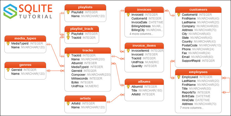
SQL relationships
In order for this recipe to work, you will need to have the sqlalchemy Python package installed. If you installed the Anaconda distribution, then it should already be available to you. SQLAlchemy is the preferred pandas tool when making connections to databases. In this recipe, you will learn how to connect to a SQLite database. You will then ask two different queries, and answer them by joining together tables with the .merge method.
How to do it…
- Before we can begin reading tables from the chinook database, we need to set up our SQLAlchemy engine:
>>> from sqlalchemy import create_engine >>> engine = create_engine('sqlite:///data/chinook.db') - We can now step back into the world of pandas and remain there for the rest of the recipe. Let's complete a command and read in the
trackstable with theread_sql_tablefunction. The name of the table is the first argument and the SQLAlchemy engine is the second:>>> tracks = pd.read_sql_table('tracks', engine) >>> tracks TrackId ... UnitPrice 0 1 ... 0.99 1 2 ... 0.99 2 3 ... 0.99 3 4 ... 0.99 4 5 ... 0.99 ... ... ... ... 3498 3499 ... 0.99 3499 3500 ... 0.99 3500 3501 ... 0.99 3501 3502 ... 0.99 3502 3503 ... 0.99 - For the rest of the recipe, we will answer a couple of different specific queries with help from the database diagram. To begin, let's find the average length of song per genre:
>>> (pd.read_sql_table('genres', engine) ... .merge(tracks[['GenreId', 'Milliseconds']], ... on='GenreId', how='left') ... .drop('GenreId', axis='columns') ... ) Name Milliseconds 0 Rock 343719 1 Rock 342562 2 Rock 230619 3 Rock 252051 4 Rock 375418 ... ... ... 3498 Classical 286741 3499 Classical 139200 3500 Classical 66639 3501 Classical 221331 3502 Opera 174813 - Now we can easily find the average length of each song per genre. To help ease interpretation, we convert the
Millisecondscolumn to thetimedeltadata type:>>> (pd.read_sql_table('genres', engine) ... .merge(tracks[['GenreId', 'Milliseconds']], ... on='GenreId', how='left') ... .drop('GenreId', axis='columns') ... .groupby('Name') ... ['Milliseconds'] ... .mean() ... .pipe(lambda s_: pd.to_timedelta(s_, unit='ms') ... .rename('Length')) ... .dt.floor('s') ... .sort_values() ... ) Name Rock And Roll 00:02:14 Opera 00:02:54 Hip Hop/Rap 00:02:58 Easy Listening 00:03:09 Bossa Nova 00:03:39 ... Comedy 00:26:25 TV Shows 00:35:45 Drama 00:42:55 Science Fiction 00:43:45 Sci Fi & Fantasy 00:48:31 Name: Length, Length: 25, dtype: timedelta64[ns] - Now let's find the total amount spent per customer. We will need the
customers,invoices, andinvoice_itemstables all connected to each other:>>> cust = pd.read_sql_table('customers', engine, ... columns=['CustomerId','FirstName', ... 'LastName']) >>> invoice = pd.read_sql_table('invoices', engine, ... columns=['InvoiceId','CustomerId']) >>> invoice_items = pd.read_sql_table('invoice_items', engine, ... columns=['InvoiceId', 'UnitPrice', 'Quantity']) >>> (cust ... .merge(invoice, on='CustomerId') ... .merge(invoice_items, on='InvoiceId') ... ) CustomerId FirstName ... UnitPrice Quantity 0 1 Luís ... 1.99 1 1 1 Luís ... 1.99 1 2 1 Luís ... 0.99 1 3 1 Luís ... 0.99 1 4 1 Luís ... 0.99 1 ... ... ... ... ... ... 2235 59 Puja ... 0.99 1 2236 59 Puja ... 0.99 1 2237 59 Puja ... 0.99 1 2238 59 Puja ... 0.99 1 2239 59 Puja ... 0.99 1 - We can now multiply the quantity by the unit price and then find the total amount spent per customer:
>>> (cust
...     .merge(invoice, on='CustomerId')
...     .merge(invoice_items, on='InvoiceId')
...     .assign(Total=lambda df_:df_.Quantity * df_.UnitPrice)
...     .groupby(['CustomerId', 'FirstName', 'LastName'])
...     ['Total']
...     .sum()
...     .sort_values(ascending=False)
... )
CustomerId  FirstName  LastName
6           Helena     Holý          49.62
26          Richard    Cunningham    47.62
57          Luis       Rojas         46.62
46          Hugh       O'Reilly      45.62
45          Ladislav   Kovács        45.62
                                     ...
32          Aaron      Mitchell      37.62
31          Martha     Silk          37.62
29          Robert     Brown         37.62
27          Patrick    Gray          37.62
59          Puja       Srivastava    36.64
Name: Total, Length: 59, dtype: float64
How it works…
The create_engine function requires a connection string to work properly. The connection string for SQLite is the location of the database, which is located in the data directory. Other relational database management systems have more complex connection strings. You will need to provide a username, password, hostname, port, and optionally, a database. You will also need to supply the SQL dialect and the driver. The general form for the connection string is as follows: dialect+driver://username:password@host:port/database. The driver for your particular relational database might need to be installed separately.
Once we have created the engine, selecting entire tables into DataFrames is very easy with the read_sql_table function in step 2. Each of the tables in the database has a primary key identifying each row. It is identified graphically with a key symbol in the diagram. In step 3, we link genres to tracks through GenreId. As we only care about the track length, we trim the tracks DataFrame down to just the columns we need before performing the merge. Once the tables have merged, we can answer the query with a basic .groupby operation.
We go one step further and convert the integer milliseconds into a Timedelta object that is far easier to read. The key is passing in the correct unit of measurement as a string. Now that we have a Timedelta Series, we can use the .dt attribute to access the .floor method, which rounds the time down to the nearest second.
The query required to answer step 5 involves three tables. We can trim the tables down significantly to only the columns we need by passing them to the columns parameter. When using .merge, the joining columns are not kept when they have the same name. In step 6, we could have assigned a column for the price times quantity with the following:
cust_inv['Total'] = cust_inv['Quantity'] * cust_inv['UnitPrice']
As has been emphasized through this book, we prefer chaining operations when possible, and hence you see .assign used frequently.
There's more…
If you are adept with SQL, you can write a SQL query as a string and pass it to the read_sql_query function. For example, the following will reproduce the output from step 4:
>>> sql_string1 = '''
... SELECT
...     Name,
...     time(avg(Milliseconds) / 1000, 'unixepoch') as avg_time
... FROM (
...       SELECT
...           g.Name,
...           t.Milliseconds
...       FROM
...           genres as g
...       JOIN
...           tracks as t on
...           g.genreid == t.genreid
...      )
... GROUP BY Name
... ORDER BY avg_time'''
>>> pd.read_sql_query(sql_string1, engine)
                Name  avg_time
0      Rock And Roll  00:02:14
1              Opera  00:02:54
2        Hip Hop/Rap  00:02:58
3     Easy Listening  00:03:09
4         Bossa Nova  00:03:39
..               ...       ...
20            Comedy  00:26:25
21          TV Shows  00:35:45
22             Drama  00:42:55
23   Science Fiction  00:43:45
24  Sci Fi & Fantasy  00:48:31
To reproduce the answer from step 6, use the following SQL query:
>>> sql_string2 = '''
...    SELECT
...          c.customerid,
...          c.FirstName,
...          c.LastName,
...          sum(ii.quantity * ii.unitprice) as Total
...    FROM
...         customers as c
...    JOIN
...         invoices as i
...         on c.customerid = i.customerid
...    JOIN
...        invoice_items as ii
...        on i.invoiceid = ii.invoiceid
...    GROUP BY
...        c.customerid, c.FirstName, c.LastName
...    ORDER BY
...        Total desc'''
>>> pd.read_sql_query(sql_string2, engine)
    CustomerId FirstName    LastName  Total
0            6    Helena        Holý  49.62
1           26   Richard  Cunningham  47.62
2           57      Luis       Rojas  46.62
3           45  Ladislav      Kovács  45.62
4           46      Hugh    O'Reilly  45.62
..         ...       ...         ...    ...
54          53      Phil      Hughes  37.62
55          54     Steve      Murray  37.62
56          55      Mark      Taylor  37.62
57          56     Diego   Gutiérrez  37.62
58          59      Puja  Srivastava  36.64