
Hadoop is an open-source framework for large-scale data storage and distributed computing, built on the MapReduce model. Doug Cutting initially created Hadoop as a component of the Nutch web crawler. It became its own project in 2006, and graduated to a top-level Apache project in 2008. During this time, Hadoop has experienced widespread adoption.
One of Hadoop’s strengths is that it is a general framework, applicable to a variety of domains and programming languages. One use case, and the common thread of the book’s remaining chapters, is to drive large R jobs.
This chapter explains some basics of MapReduce and Hadoop. It may feel a little out of place, as it’s not specific to R; but the content is too important to hide in an appendix.
Have no fear: I don’t dive into deep details here. There is a lot more to MapReduce and Hadoop than I could possibly cover in this book, let alone a chapter. I’ll provide just enough guidance to set you on your way. For a more thorough exploration I encourage you to read the Google MapReduce paper mentioned in , as well as Hadoop: The Definitive Guide by Tom White (O’Reilly).
If you already have a grasp on MapReduce and Hadoop, feel free to skip to the next chapter.
When people think “Apache Hadoop,”[43] they often think about churning through terabytes of input across clusters made of tens or hundreds of machines, or nodes. Logfile processing is such an oft-cited use case, in fact, that Hadoop virgins may think this is all the tool is good for. That would be an unfortunately narrow view of Hadoop’s capabilities.
Plain and simple, Hadoop is a framework for parallel processing: decompose a problem into independent units of work, and Hadoop will distribute that work across a cluster of machines. This means you get your results back much faster than if you had run each unit of work sequentially, on a single machine. Hadoop has proven useful for extract-transform-load (ETL) work, image processing, data analysis, and more.
While Hadoop’s parallel processing muscle is suitable for large amounts of data, it is equally useful for problems that involve large amounts of computation (sometimes known as “processor-intensive” or “CPU-intensive” work). Consider a program that, based on a handful of input values, runs for some tens of minutes or even a number of hours: if you needed to test several variations of those input values, then you would certainly benefit from a parallel solution.
Hadoop’s parallelism is based on the MapReduce model. To understand how Hadoop can boost your R performance, then, let’s first take a quick look at MapReduce.
The MapReduce model outlines a way to perform work across a cluster built of inexpensive, commodity machines. It was popularized by Google in a paper, “MapReduce: Simplified Data Processing on Large Clusters” by Jeffrey Dean and Sanjay Ghemawat.[44] Google built their own implementation to churn web content, but MapReduce has since been applied to other pursuits.
The name comes from the model’s two phases, Map and Reduce. Consider that you start with a single mountain of input. In the Map phase, you divide that input and group the pieces into smaller, independent piles of related material. Next, in the Reduce phase, you perform some action on each pile. (This is why we describe MapReduce as a “divide-and-conquer” model.) The piles can be Reduced in parallel because they do not rely on one another.
A simplified version of a MapReduce job proceeds as follows:
Map Phase
Each cluster node takes a piece of the initial mountain of data and runs a Map task on each record (item) of input. You supply the code for the Map task.
The Map tasks all run in parallel, creating a key/value pair for each record. The key identifies the item’s pile for the reduce operation. The value can be the record itself or some derivation thereof.
The Shuffle
At the end of the Map phase, the machines all pool their results. Every key/value pair is assigned to a pile, based on the key. (You don’t supply any code for the shuffle. All of this is taken care of for you, behind the scenes.)[45]
Reduce Phase
The cluster machines then switch roles and run the Reduce task on each pile. You supply the code for the Reduce task, which gets the entire pile (that is, all of the key/value pairs for a given key) at once.
The Reduce task typically, but not necessarily, emits some output for each pile.
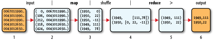
Figure 5-1 provides a visual representation of a
MapReduce flow.[46] Consider an input for which each line is a record of format
(letter)(number), and the goal is to
find the maximum value of (number) for
each (letter). (The figure only shows
letters A, B, and C, but you could imagine this covers all letters A
through Z.) Cell (1) depicts the raw input. In cell (2), the MapReduce
system feeds each record’s line number and content to the Map process,
which decomposes the record into a key (letter) and value (number). The Shuffle step gathers all of the
values for each letter into a common bucket, and feeds each bucket to the
Reduce step. In turn, the Reduce step plucks out the maximum value from
the bucket. The output is a set of (letter),(maximum number) pairs.
This may still feel a little abstract. A few examples should help firm this up.
Sometimes the toughest part of using Hadoop is trying to express a problem in MapReduce terms. Since the payoff—scalable, parallel processing across a farm of commodity hardware—is so great, it’s often worth the extra mental muscle to convince a problem to fit the MapReduce model.
Let’s walk through some pseudocode for the Map and Reduce tasks, and how they handle key/value pairs. Note that there is a special case in which you can have a Map-only job for simple parallelization. (I’ll cover real code in the next chapters, as each Hadoop-related solution I present has its own ways of talking MapReduce.)
For these examples, I’ll use a fictitious text input format in which each record is a comma-separated line that describes a phone call:
{date},{caller num},{caller carrier},{dest num},{dest carrier},{length}This uses the Map task to group the records by day, then calculates the mean (average) call length in the Reduce task.
Map task
Receives a single line of input (that is, one input record)
Uses text manipulation to extract the
{date}and{length}fieldsEmits key:
{date}, value:{length}
Reduce task
Receives key:
{date}, values:{length1 … lengthN}(that is, each reduce task receives all of the call lengths for a single date)Loops through
{length1 …
          lengthN}
to calculate total call length, and also to note the number of callsCalculates the mean (divides the total call length by the number of calls)
Outputs the date and the mean call length
This time, the goal is to get a breakdown of each caller for each date. The Map phase will define the keys to group the inputs, and the Reduce task will perform the calculations. Notice that the Map task emits a dummy value (the number 1) as its value because we use the Reduce task for a simple counting operation.
Map task
Receives single line of input
Uses text manipulation to extract
{date},{caller num}Emits key:
{date}{caller
          num}
, value:1
Reduce task
Receives key:
{date}{caller
          num}
, value:{1 … 1}Loops through each item, to count total number of items (calls)
Outputs
{date},{caller num}and the number of calls
In this last case, there’s no need to group the input records; we simply wish to run some special function for every input record. Because the Map phase runs in parallel across the cluster, we can leverage MapReduce to execute some (possibly long-running) code for each input record and reap the time-saving parallel execution.
Chances are, this is how you will run a good deal of your R code through Hadoop.
Map task
Receives single line of input
Uses text manipulation to extract function parameters
Passes those parameters to a potentially long-running function
Emits key:
{function
          output}
, value:{null}
(There is no Reduce task.)
Earlier, I oversimplified Hadoop processing when I explained that input records are lines of delimited text. If you expect that all of your input will be of this form, feel free to skip this section. You’re in quite a different boat if you plan to use Hadoop with binary data (sound files, image files, proprietary data formats) or if you want to treat an entire text file (XML document) as a record.
By default, when you point Hadoop to an input file, it will assume it is a text document and treat each line as a record. There are times when this is not what you want: maybe you’re performing feature extraction on sound files, or you wish to perform sentiment analysis on text documents. How do you tell Hadoop to work on the entire file, be it binary or text?
The answer is to use a special archive called a SequenceFile.[47] A SequenceFile is similar to a zip or tar file, in that it’s just a container for other files. Hadoop considers each file in a SequenceFile to be its own record.
To manage zip files, you use the zip command. Tar file? Use tar. SequenceFiles? Hadoop doesn’t ship with any
tools for this, but you still have options: you can write a Hadoop job
using the Java API; or you can use the forqlift command-line tool. Please see the
sidebar for
details.
The techniques presented in the next three chapters all require that you have a Hadoop cluster at your disposal. Your company may already have one, in which case you’ll want to talk to your Hadoop admins to get connection details.
If your company doesn’t have a Hadoop cluster, or you’re working on your own, you can build one using Amazon’s cloud computing wing, Amazon Web Services (AWS).[48] Setting up a Hadoop cluster in the AWS cloud would merit a book on its own, so we can only provide some general guidance here. Please refer to Amazon’s documentation for details.
AWS provides computing resources such as virtual servers and storage in metered (pay-per-use) fashion. Customers benefit from fast ramp-up time, zero commitment, and no up-front infrastructure costs compared to traditional datacenter computing. These factors make AWS especially appealing to individuals, start-ups, and small firms.
You can hand-build your cluster using virtual servers on Elastic Compute Cloud (EC2), or you can leverage the Hadoop-on-demand service called Elastic MapReduce (EMR).
Building on EC2 means having your own Hadoop cluster in the cloud. You get complete control over the node configuration and long-term storage in the form of HDFS, Hadoop’s distributed filesystem. This comes at the expense of doing a lot more grunt work up-front and having to know more about systems administration on EC2. The Apache Whirr project[49] provides tools to ease the burden, but there’s still no free lunch here.
By comparison, EMR is as simple and hands-off as it gets: tell AWS how many nodes you want, what size (instance type) they should be, and you’re off to the races. EMR’s value-add is that AWS will build the cluster for you, on-demand, and run your job. You only pay for data storage, and for machine time while the cluster is running. The trade-off is that, as of this writing, you don’t get to choose which machine image (AMI) to use for the cluster nodes. Amazon deploys its own AMI, currently based on Debian 5, Hadoop 0.20.0, and R 2.7. You have (limited) avenues for customization through EMR “bootstrap action” scripts. While it’s possible to upgrade R and install some packages, this gets to be a real pain because you have to do that every time you launch a cluster.
When I say “each time,” I mean that an EMR-based cluster is designed
to be ephemeral: by default, AWS tears down the cluster as soon as your
job completes. All of the cluster nodes and resources disappear. That
means you can’t leverage HDFS for long-term storage. If you plan to run a
series of jobs in short order, pass the --alive flag on cluster creation and the cluster
will stay alive until you manually shut it down. Keep in mind, though,
this works against one of EMR’s perks: you’ll continue to incur cost as
long as the cluster is running, even if you forget to turn it off.
Your circumstances will tell you whether to choose EC2 or EMR. The greater your desire to customize the Hadoop cluster, the more you should consider building out a cluster on EC2. This requires more up-front work and incurs greater runtime cost, but allows you to have a true Hadoop cluster (complete with HDFS). That makes the EC2 route more suitable for a small company that has a decent budget and dedicated sysadmins for cluster administration. If you lack the time, inclination, or skill to play sysadmin, then EMR is your best bet. Sure, running bootstrap actions to update R is a pain, but it still beats the distraction of building your own EC2 cluster.
In either case, the economics of EC2 and EMR lower Hadoop’s barrier to entry. One perk of a cloud-based cluster is that the return-on-investment (ROI) calculations are very different from those of a physical cluster, where you need to have a lot of Hadoop-able “big-data” work to justify the expense. By comparison, a cloud cluster opens the door to using Hadoop on “medium-data” problems.
In this chapter, I’ve explained MapReduce and its implementation in Apache Hadoop. Along the way, I’ve given you a start on building your own Hadoop cluster in the cloud. I also oversimplified a couple of concepts so as to not drown you in detail. I’ll pick up on a couple of finer points in the next chapter, when I discuss mixing Hadoop and R: I call it, quite simply, R+Hadoop.
[45] Well, you can provide code to influence the shuffle phase, under certain advanced cases. Please refer to Hadoop: The Definitive Guide for details.
[46] A hearty thanks to Tom White for letting us borrow and modify this diagram from his book.
[47] There’s another reason you want to use a SequenceFile, but it’s not really an issue for this book. The curious among you can take a gander at Tom White’s explanation in “The Small Files Problem,” at http://www.cloudera.com/blog/2009/02/the-small-files-problem/.