In order to execute any functions in parallel with snow, you must first create a cluster object. The cluster object is used to interact with the cluster workers, and is passed as the first argument to many of the snow functions. You can create different types of cluster objects, depending on the transport mechanism that you wish to use.

The basic cluster creation function is makeCluster() which can create any type of cluster. Let’s use it to create a cluster of four workers on the local machine using the socket transport:

cl <- makeCluster(4, type="SOCK")

The first argument is the cluster specification, and the second is the cluster type. The interpretation of the cluster specification depends on the type, but all cluster types allow you to specify a worker count.

Socket clusters also allow you to specify the worker machines as a character vector. The following will launch four workers on remote machines:

spec <- c("n1", "n2", "n3", "n4")
cl <- makeCluster(spec, type="SOCK")

The socket transport launches each of these workers via the ssh command^[6] unless the name is “localhost”, in which case makeCluster() starts the worker itself. For remote execution, you should configure ssh to use password-less login. This can be done using public-key authentication and SSH agents, which is covered in chapter 6 of SSH, The Secure Shell: The Definitive Guide (O’Reilly) and many websites.

makeCluster() allows you to specify addition arguments as configuration options. This is discussed further in snow Configuration.

The type argument can be “SOCK”, “MPI”, “PVM” or “NWS”. To create an MPI cluster with four workers, execute:

cl <- makeCluster(4, type="MPI")

This will start four MPI workers on the local machine unless you make special provisions, as described in the section Executing snow Programs on a Cluster with Rmpi.

You can also use the functions makeSOCKcluster(), makeMPIcluster(), makePVMcluster(), and makeNWScluster() to create specific types of clusters. In fact, makeCluster() is nothing more than a wrapper around these functions.

To shut down any type of cluster, use the stopCluster() function:

stopCluster(cl)

Some cluster types may be automatically stopped when the R session exits, but it’s good practice to always call stopCluster() in snow scripts; otherwise, you risk leaking cluster workers if the cluster type is changed, for example.

We’re finally ready to use snow to do some parallel computing, so let’s look at a real example: parallel K-Means. K-Means is a clustering algorithm that partitions rows of a dataset into k clusters.^[7] It’s an iterative algorithm, since it starts with a guess of the location for each of the cluster centers, and gradually improves the center locations until it converges on a solution.

R includes a function for performing K-Means clustering in the stats package: the kmeans() function. One way of using the kmeans() function is to specify the number of cluster centers, and kmeans() will pick the starting points for the centers by randomly selecting that number of rows from your dataset. After it iterates to a solution, it computes a value called the total within-cluster sum of squares. It then selects another set of rows for the starting points, and repeats this process in an attempt to find a solution with a smallest total within-cluster sum of squares.

Let’s use kmeans() to generate four clusters of the “Boston” dataset, using 100 random sets of centers:

library(MASS)
result <- kmeans(Boston, 4, nstart=100)

We’re going to take a simple approach to parallelizing kmeans() that can be used for parallelizing many similar functions and doesn’t require changing the source code for kmeans(). We simply call the kmeans() function on each of the workers using a smaller value of the nstart argument. Then we combine the results by picking the result with the smallest total within-cluster sum of squares.

But before we execute this in parallel, let’s try using this technique using the lapply() function to make sure it works. Once that is done, it will be fairly easy to convert to one of the snow parallel execution functions:

library(MASS)
results <- lapply(rep(25, 4), function(nstart) kmeans(Boston, 4, nstart=nstart))
i <- sapply(results, function(result) result$tot.withinss)
result <- results[[which.min(i)]]

We used a vector of four 25s to specify the nstart argument in order to get equivalent results to using 100 in a single call to kmeans(). Generally, the length of this vector should be equal to the number of workers in your cluster when running in parallel.

Now let’s parallelize this algorithm. snow includes a number of functions that we could use, including clusterApply(), clusterApplyLB(), and parLapply(). For this example, we’ll use clusterApply(). You call it exactly the same as lapply(), except that it takes a snow cluster object as the first argument. We also need to load MASS on the workers, rather than on the master, since it’s the workers that use the “Boston” dataset.

Assuming that snow is loaded and that we have a cluster object named cl, here’s the parallel version:

ignore <- clusterEvalQ(cl, {library(MASS); NULL})
results <- clusterApply(cl, rep(25, 4), function(nstart) kmeans(Boston, 4, 
    nstart=nstart))
i <- sapply(results, function(result) result$tot.withinss)
result <- results[[which.min(i)]]

clusterEvalQ() takes two arguments: the cluster object, and an expression that is evaluated on each of the workers. It returns the result from each of the workers in a list, which we don’t use here. I use a compound expression to load MASS and return NULL to avoid sending unnecessary data back to the master process. That isn’t a serious issue in this case, but it can be, so I often return NULL to be safe.

As you can see, the snow version isn’t that much different than the lapply() version. Most of the work was done in converting it to use lapply(). Usually the biggest problem in converting from lapply() to one of the parallel operations is handling the data properly and efficiently. In this case, the dataset was in a package, so all we had to do was load the package on the workers.

In the last section we used the clusterEvalQ() function to initialize the cluster workers by loading a package on each of them. clusterEvalQ() is very handy, especially for interactive use, but it isn’t very general. It’s great for executing a simple expression on the cluster workers, but it doesn’t allow you to pass any kind of parameters to the expression, for example. Also, although you can use it to execute a function, it won’t send that function to the worker first,^[9] as clusterApply() does.

My favorite snow function for initializing the cluster workers is clusterCall(). The arguments are pretty simple: it takes a snow cluster object, a worker function, and any number of arguments to pass to the function. It simply calls the function with the specified arguments on each of the cluster workers, and returns the results as a list. It’s like clusterApply() without the x argument, so it executes once for each worker, like clusterEvalQ(), rather than once for each element in x.

clusterCall() can do anything that clusterEvalQ() does and more.^[10] For example, here’s how we could use clusterCall() to load the MASS package on the cluster workers:

clusterCall(cl, function() { library(MASS); NULL })

This defines a simple function that loads the MASS package and returns NULL.^[11] Returning NULL guarantees that we don’t accidentally send unnecessary data transfer back to the master.^[12]

The following will load several packages specified by a character vector:

worker.init <- function(packages) {
  for (p in packages) {
    library(p, character.only=TRUE)
  }
  NULL
}
clusterCall(cl, worker.init, c('MASS', 'boot'))

Setting the character.only argument to TRUE makes library() interpret the argument as a character variable. If we didn’t do that, library() would attempt to load a package named p repeatedly.

Although it’s not as commonly used as clusterCall(), the clusterApply() function is also useful for initializing the cluster workers since it can send different data to the initialization function for each worker. The following creates a global variable on each of the cluster workers that can be used as a unique worker ID:

clusterApply(cl, seq(along=cl), function(id) WORKER.ID <<- id)

We introduced the clusterApply() function in the parallel K-Means example. The next parallel execution function that I’ll discuss is clusterApplyLB(). It’s very similar to clusterApply(), but instead of scheduling tasks in a round-robin fashion, it sends new tasks to the cluster workers as they complete their previous task. By round-robin, I mean that clusterApply() distributes the elements of x to the cluster workers one at a time, in the same way that cards are dealt to players in a card game. In a sense, clusterApply() (politely) pushes tasks to the workers, while clusterApplyLB() lets the workers pull tasks as needed. That can be more efficient if some tasks take longer than others, or if some cluster workers are slower.

To demonstrate clusterApplyLB(), we’ll execute Sys.sleep() on the workers, giving us complete control over the task lengths. Since our real interest in using clusterApplyLB() is to improve performance, we’ll use snow.time() to gather timing information about the overall execution.^[13] We will also use snow.time()’s plotting capability to visualize the task execution on the workers:

set.seed(7777442)
sleeptime <- abs(rnorm(10, 10, 10))
tm <- snow.time(clusterApplyLB(cl, sleeptime, Sys.sleep))
plot(tm)

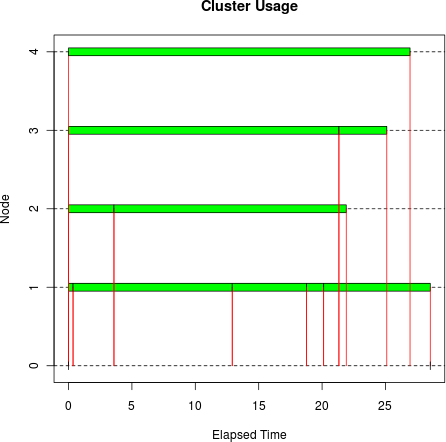
Ideally there would be solid horizontal bars for nodes 1 through 4 in the plot, indicating that the cluster workers were always busy, and therefore running efficiently. clusterApplyLB() did pretty well, although there was some wasted time at the end.

Now let’s try the same problem with clusterApply():^[14]

set.seed(7777442)
sleeptime <- abs(rnorm(10, 10, 10))
tm <- snow.time(clusterApply(cl, sleeptime, Sys.sleep))
plot(tm)

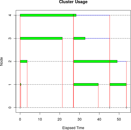
As you can see, clusterApply() is much less efficient than clusterApplyLB() in this example: it took 53.7 seconds, versus 28.5 seconds for clusterApplyLB(). The plot shows how much time was wasted due to the round-robin scheduling.

But don’t give up on clusterApply(): it has its uses. It worked fine in the parallel K-Means example because we had the same number of tasks as workers. It is also used to implement the very useful parLapply() function, which we will discuss next.^[15]

Now that we’ve discussed and compared clusterApply() and clusterApplyLB(), let’s consider parLapply(), a third parallel lapply() function that has the same arguments and basic behavior as clusterApply() and clusterApplyLB(). But there is an important difference that makes it perhaps the most generally useful of the three.

parLapply() is a high-level snow function, that is actually a deceptively simple function wrapping an invocation of clusterApply():

> parLapply
function (cl, x, fun, ...)
docall(c, clusterApply(cl, splitList(x, length(cl)), lapply, fun, ...))
<environment: namespace:snow>

Basically, parLapply() splits up x into a list of subvectors, and processes those subvectors on the cluster workers using lapply(). In effect, it is prescheduling the work by dividing the tasks into as many chunks as there are workers in the cluster. This is functionally equivalent to using clusterApply() directly, but it can be much more efficient, since there are fewer I/O operations between the master and the workers. If the length of x is already equal to the number of workers, then parLapply() has no advantage. But if you’re parallelizing an R script that already uses lapply(), the length of x is often very large, and at any rate is completely unrelated to the number of workers in your cluster. In that case, parLapply() is a better parallel version of lapply() than clusterApply().

One way to think about it is that parLapply() interprets the x argument differently than clusterApply(). clusterApply() is low-level, and treats x as a specification of the tasks to execute on the cluster workers using fun. parLapply() treats x as a source of disjoint input arguments to execute on the cluster workers using lapply() and fun. clusterApply() gives you more control over what gets sent to who, while parLapply() provides a convenient way to efficiently divide the work among the cluster workers.

An interesting consequence of parLapply()’s work scheduling is that it is much more efficient than clusterApply() if you have many more tasks than workers, and one or more large, additional arguments to pass to parLapply(). In that case, the additional arguments are sent to each worker only once, rather than possibly many times. Let’s try doing that, using a slightly altered parallel sleep function that takes a matrix as an argument:

bigsleep <- function(sleeptime, mat) Sys.sleep(sleeptime)
bigmatrix <- matrix(0, 2000, 2000)
sleeptime <- rep(1, 100)

I defined the sleeptimes to be small, many, and equally sized. This will accentuate the performance differences between clusterApply() and parLapply():

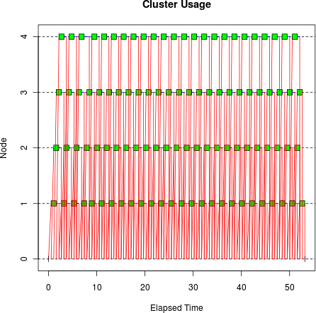
tm <- snow.time(clusterApply(cl, sleeptime, bigsleep, bigmatrix))
plot(tm)

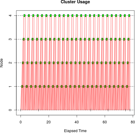
This doesn’t look very efficient: you can see that there are many sends and receives between the master and the workers, resulting in relatively big gaps between the compute operations on the cluster workers. The gaps aren’t due to load imbalance as we saw before: they’re due to I/O time. We’re now spending a significant fraction of the elapsed time sending data to the workers, so instead of the ideal elapsed time of 25 seconds,^[16] it’s taking 77.9 seconds.

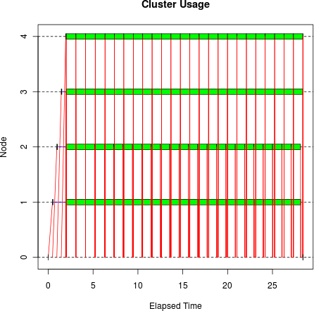
Now let’s do the same thing using parLapply():

tm <- snow.time(parLapply(cl, sleeptime, bigsleep, bigmatrix))
plot(tm)

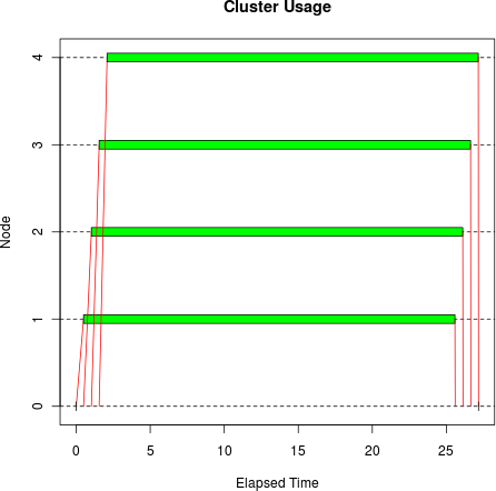
The difference is dramatic, both visually and in elapsed time: it took only 27.2 seconds, beating clusterApply() by 50.7 seconds.

Keep in mind that this particular use of clusterApply() is bad: it is needlessly sending the matrix to the worker with every task. There are various ways to fix that, and using parLapply() happens to work well in this case. On the other hand, if you’re sending huge objects in x, then there’s not much you can do, and parLapply() isn’t going to help. My point is that parLapply() schedules work in a useful and efficient way, making it probably the single most useful parallel execution function in snow. When in doubt, use parLapply().

In the previous section I showed you how parLapply() uses clusterApply() to implement a parallel operation that solves a certain class of parallel program quite nicely. Recall that parLapply() executes a user-supplied function for each element of x just like clusterApply(). But what if we want the function to operate on subvectors of x? That’s similar to what parLapply() does, but is a bit easier to implement, since it doesn’t need to use lapply() to call the user’s function.

We could use the splitList() function, like parLapply() does, but that is a snow internal function. Instead, we’ll use the clusterSplit() function which is very similar, and slightly more convenient. Let’s try splitting the sequence from 1 to 30 for our cluster using clusterSplit():

> clusterSplit(cl, 1:30)
[[1]]
[1] 1 2 3 4 5 6 7 8

[[2]]
[1]  9 10 11 12 13 14 15

[[3]]
[1] 16 17 18 19 20 21 22

[[4]]
[1] 23 24 25 26 27 28 29 30

Since our cluster has four workers, it splits the sequence into a list of four nearly equal length vectors, which is just what we need.

Now let’s define parVapply() to split x using clusterSplit(), execute the user function on each of the pieces using clusterApply(), and combine the results using do.call() and c():

parVapply <- function(cl, x, fun, ...) {
  do.call("c", clusterApply(cl, clusterSplit(cl, x), fun, ...))
}

Like parLapply(), parVapply() always issues the same number of tasks as workers. But unlike parLapply(), the user-supplied function is only executed once per worker. Let’s use parVapply() to compute the cube root of numbers from 1 to 10 using the ^ function:

> parVapply(cl, 1:10, "^", 1/3)
 [1] 1.000000 1.259921 1.442250 1.587401 1.709976 1.817121 1.912931 2.000000
 [9] 2.080084 2.154435

This works because the ^ function takes a vector as its first argument and returns a vector of the same length.^[17]

We’ve talked about the advantages of parLapply() over clusterApply() at some length. In particular, when there are many more tasks than cluster workers and the task objects sent to the workers are large, there can be serious performance problems with clusterApply() that are solved by parLapply(). But what if the task execution has significant variation so that we need load balancing? clusterApplyLB() does load balancing, but would have the same performance problems as clusterApply(). We would like a load balancing equivalent to parLapply(), but there isn’t one—so let’s write it.^[18]

In order to achieve dynamic load balancing, it helps to have a number of tasks that is at least a small integer multiple of the number of workers. That way, a long task assigned to one worker can be offset by many shorter tasks being done by other workers. If that is not the case, then the other workers will sit idle while the one worker completes the long task. parLapply() creates exactly one task per worker, which is not what we want in this case. Instead, we’ll first send the function and the fixed arguments to the cluster workers using clusterCall(), which saves them in the global environment, and then send the varying argument values using clusterApplyLB(), specifying a function that will execute the user-supplied function along with the full collection of arguments.

Here are the function definitions for parLapplyLB() and the two functions that it executes on the cluster workers:

parLapplyLB <- function(cl, x, fun, ...) {
  clusterCall(cl, LB.init, fun, ...)
  r <- clusterApplyLB(cl, x, LB.worker)
  clusterEvalQ(cl, rm('.LB.fun', '.LB.args', pos=globalenv()))
  r
}
LB.init <- function(fun, ...) {
  assign('.LB.fun', fun, pos=globalenv())
  assign('.LB.args', list(...), pos=globalenv())
  NULL
}
LB.worker <- function(x) {
  do.call('.LB.fun', c(list(x), .LB.args))
}

parLapplyLB() initializes the workers using clusterCall(), executes the tasks with clusterApplyLB(), cleans up the global environment of the cluster workers with clusterEvalQ(), and finally returns the task results.

That’s all there is to implementing a simple and efficient load balancing parallel execution function. Let’s compare clusterApplyLB() to parLapplyLB() using the same test function that we used to compare clusterApply() and parLapply(), starting with clusterApplyLB():

bigsleep <- function(sleeptime, mat) Sys.sleep(sleeptime)
bigmatrix <- matrix(0, 2000, 2000)
sleeptime <- rep(1, 100)
tm <- snow.time(clusterApplyLB(cl, sleeptime, bigsleep, bigmatrix))
plot(tm)

There are lots of gaps in the execution bars due to high I/O time: the master is barely able to supply the workers with tasks. Obviously this problem isn’t going to scale to many more workers.

Now let’s try our new parLapplyLB() function:

tm <- snow.time(parLapplyLB(cl, sleeptime, bigsleep, bigmatrix))
plot(tm)

That took only 28.4 seconds versus 53.2 seconds for clusterApplyLB().

Notice that the first task on each worker has a short execution time, but a long task send time, as seen by the slope of the first four lines between the master (node 0) and the workers (nodes 1-4). Those are the worker initialization tasks executed by clusterCall() that send the large matrix to the workers. The tasks executed via clusterApplyLB() were more efficient, as seen by the vertical communication lines and the solid horizontal bars.

Most of the parallel execution functions in snow take a function object as an argument, which I call the worker function, since it is sent to the cluster workers, and subsequently executed by them. In order to send it to the workers, the worker function must be serialized into a stream of bytes using the serialize() function.^[19] That stream of bytes is converted into a copy of the original object using the unserialize() function.

In addition to a list of formal arguments and a body, the worker function includes a pointer to the environment in which it was created. This environment becomes the parent of the evaluation environment when the worker function is executed, giving the worker function access to non-local variables. Obviously, this environment must be serialized along with the rest of the worker function in order for the function to work properly after being unserialized.

However, environments are serialized in a special way in R. In general, the contents are included when an environment is serialized, but not always. Name space environments are serialized by name, not by value. That is, the name of the package is written to the resulting stream of bytes, not the symbols and objects contained in the environment. When a name space is unserialized, it is reconstructed by finding and loading the corresponding package. If the package cannot be loaded, then the stream of bytes cannot be unserialized. The global environment is also serialized by name, and when it is unserialized, the resulting object is simply a reference to the existing, unmodified global environment.

So what does this mean to you as a snow programmer? Basically, you must ensure that all the variables needed to execute the worker function are available after it has been unserialized on the cluster workers. If the worker function’s environment is the global environment and the worker function needs to access any variables in it, you need to send those variables to the workers explicitly. This can be done, for example, by using the clusterExport() function. But if the worker function was created by another function, its environment is the evaluation environment of the creator function when the worker function was created. All the variables in this environment will be serialized along with the worker function, and accessible to it when it is executed by the cluster workers. This can be a handy way of making variables available to the worker function, but if you’re not careful, you could accidentally serialize large, unneeded objects along with the worker function, causing performance to suffer. Also, if you want the worker function to use any of the creator function’s arguments, you need to evaluate those arguments before calling parLapply() or clusterApplyLB(); otherwise, you may not be able to evaluate them successfully on the workers due to R’s lazy argument evaluation.

Let’s look at a few examples to illustrate some of these issues. We’ll start with a script that multiplies a vector x by a sequence of numbers:

a <- 1:4
x <- rnorm(4)
clusterExport(cl, "x")
mult <- function(s) s * x
parLapply(cl, a, mult)

In this script, the function mult() is defined at the top level, so its environment is the global environment.^[20] Thus, x isn’t serialized along with mult(), so we need to send it to the cluster workers using the clusterExport() function. Of course, a more natural solution in this case would be to include x as an explicit argument to mult(), and then parLapply() would send it to the workers for us. However, using clusterExport() could be more efficient if we were going to reuse x by calling mult() many times with parLapply().

Now let’s turn part of this script into a function. Although this change may seem trivial, it actually changes the way mult() is serialized in parLapply():

pmult <- function(cl) {
  a <- 1:4
  x <- rnorm(4)
  mult <- function(s) s * x
  parLapply(cl, a, mult)
}
pmult(cl)

Since mult() is created by pmult(), all of pmult()’s local variables will be accessible when mult() is executed by the cluster workers, including x. Thus, we no longer call clusterExport().

Pmult() would be more useful if the values to be multiplied weren’t hardcoded, so let’s improve it by passing a and x in as arguments:

pmult <- function(cl, a, x) {
  x  # force x
  mult <- function(s) s * x
  parLapply(cl, a, mult)
}
scalars <- 1:4
dat <- rnorm(4)
pmult(cl, scalars, dat)

At this point, you may be wondering why x is on a line by itself with the cryptic comment “force x”. Although it may look like it does nothing, this operation forces x to be evaluated by looking up the value of the variable dat (the actual argument corresponding to x that is passed to the function when pmult() is invoked) in the caller’s execution environment. R uses lazy argument evaluation, and since x is now an argument, we have to force its evaluation before calling parLapply(); otherwise, the workers will report that dat wasn’t found, since they don’t have access to the environment where dat is defined. Note that they wouldn’t say x wasn’t found: they would find x, but wouldn’t be able to evaluate it because they don’t have access to dat. By evaluating x before calling parLapply(), mult()’s environment will be serialized with x set to the value of dat, rather than the symbol dat.

Notice in this last example that, in addition to x, a and cl are also serialized along with mult(). mult() doesn’t need to access them, but since they are defined in pmult’s evaluation environment, they will be serialized along with mult(). To prevent that, we can reset the environment of mult() to the global environment and pass x to mult() explicitly:

pmult <- function(cl, a, x) {
  mult <- function(s, x) s * x
  environment(mult) <- .GlobalEnv
  parLapply(cl, a, mult, x)
}
scalars <- 1:4
dat <- rnorm(4)
pmult(cl, scalars, dat)

Of course, another way to achieve the same result is to create mult() at the top level of the script so that mult() is associated with the global environment in the first place.

Unfortunately, you run into some tricky issues when sending function objects over the network. You may conclude that you don’t want to use the worker function’s environment to send data to your cluster workers, and that’s a perfectly reasonable position. But hopefully you now understand the issues well enough to figure out what methods work best for you.

As I mentioned previously, snow is very useful for performing Monte Carlo simulations, bootstrapping, and other operations that depend on the use of random numbers. When running such operations in parallel, it’s important that the cluster workers generate different random numbers; otherwise, the workers may all replicate each other’s results, defeating the purpose of executing in parallel. Rather than using ad-hoc schemes for seeding the workers differently, it is better to use a parallel random number generator package. snow provides support for the rlecuyer and rsprng packages, both of which are available on CRAN. With one of these packages installed on all the nodes of your cluster, you can configure your cluster workers to use it via the clusterSetupRNG() function. The type argument specifies which generator to use. To use rlecuyer, set type to RNGstream:

clusterSetupRNG(cl, type='RNGstream')

To use rsprng, set type to SPRNG:

clusterSetupRNG(cl, type='SPRNG')

You can specify a seed using the seed argument. rsprng uses a single integer for the seed, while rlecuyer uses a vector of six integers:

clusterSetupRNG(cl, type='RNGstream', seed=c(1,22,333,444,55,6))

Now the standard random number functions will use the specified parallel random number generator:

> unlist(clusterEvalQ(cl, rnorm(1)))
[1] -1.0452398 -0.3579839 -0.5549331  0.7823642

If you reinitialize the cluster workers using the same seed, you will get the same random number from each of the workers.

We can also get reproducible results using clusterApply(), but not with clusterApplyLB() because clusterApply() always uses the same task scheduling, while clusterApplyLB() does not.^[21]

snow includes a number of configuration options for controlling the way the cluster is created. These options can be specified as named arguments to the cluster creation function (makeCluster(), makeSOCKcluster(), makeMPIcluster(), etc.). For example, here is the way to specify an alternate hostname for the master:

cl <- makeCluster(3, type="SOCK", master="192.168.1.100")

You can also use the setDefaultClusterOptions() function to change a default configuration option during an R session. By default, the outfile option is set to /dev/null, which causes all worker output to be redirected to the null device (the proverbial bit bucket). To prevent output from being redirected, you can change the default value of outfile to the empty string:

setDefaultClusterOptions(outfile="")

This is a useful debugging technique which we will discuss more in Troubleshooting snow Programs.

Here is a summary of all of the snow configuration options:

It is possible, although a bit tricky, to configure different workers differently. I’ve done this when running a snow program in parallel on an ad-hoc collection of workstations. In fact, there are two mechanisms available for that with the socket transport. The first approach works for all the transports. You set the homogeneous option to FALSE, which causes snow to use a special startup script to launch the workers. This alternate script doesn’t assume that the worker nodes are set up the same as the master node, but can look for R or Rscript in the user’s PATH, for example. It also supports the use of environment variables to configure the workers, such as R_SNOW_RSCRIPT_CMD and R_SNOW_LIB to specify the path of the Rscript command and the snow installation directory. These environment variables can be set to appropriate values in the user’s environment on each worker machine using the shell’s start up scripts.

The second approach to heterogeneous configuration only works with the socket and nws transports. When you call makeSOCKcluster(), you specify the worker machines as a list of lists. In this case, the hostname of the worker is specified by the host element of each sublist. The other elements of the sublists are used to override the corresponding option for that worker.

Let’s say we want to create a cluster with two workers: n1 and n2, but we need to log in as a different user on machine n2:

> workerList <- list(list(host = "n1"), list(host = "n2", user = "steve"))
> cl <- makeSOCKcluster(workerList)
> clusterEvalQ(cl, Sys.info()[["user"]])
[[1]]
[1] "weston"

[[2]]
[1] "steve"

> stopCluster(cl)

It can also be useful to set the outfile option differently to avoid file conflicts between workers:

> workerList <- list(list(host = "n1", outfile = "n1.log", user = "weston"), 
+                    list(host = "n2", outfile = "n2-1.log"), 
+                    list(host = "n2", outfile = "n2-2.log"))
> cl <- makeSOCKcluster(workerList, user = "steve")
> clusterEvalQ(cl, Sys.glob("*.log"))
[[1]]
[1] "n1.log"

[[2]]
[1] "n2-1.log" "n2-2.log"

[[3]]
[1] "n2-1.log" "n2-2.log"

> stopCluster(cl)

This also demonstrates that different methods for setting options can be used together. The machine-specific option values always take precedence.

As I mentioned previously, installing Rmpi can be problematic because it depends on MPI being previously installed. Also, there are multiple MPI distributions, and some of the older distributions have compatibility problems with Rmpi. In general, Open MPI is the preferred MPI distribution. Fortunately, Open MPI is readily available for modern Linux systems. The website for the Open MPI Project is http://www.open-mpi.org/.

Another problem is that there isn’t a binary distribution of Rmpi available for Windows. Thus, even if you have MPI installed on a Windows machine, you will also need to install Rmpi from the source distribution, which requires additional tools that may also need to be installed. For more information on installing Rmpi on Windows, see the documentation in the Rmpi package. That’s beyond the scope of this book.

Installation of Rmpi on the Mac was quite simple on Mac OS X 10.5 and 10.6, both of which came with Open MPI, but unfortunately, Apple stopped distributing it in Mac OS X 10.7. If you’re using 10.5 or 10.6, you can (hopefully) install Rmpi quite easily:^[22]

install.packages("Rmpi")

If you’re using Mac OS X 10.7, you’ll have to install Open MPI first, and then you’ll probably have to build Rmpi from the source distribution since the binary distribution probably won’t be compatible with your installation of Open MPI. I’ll discuss installing Rmpi from the source distribution shortly, but not Open MPI.

On Debian/Ubuntu, Rmpi is available in the “r-cran-rmpi” Debian package, and can be installed with apt-get. That’s the most foolproof way to install Rmpi on Ubuntu, for example, since apt-get will automatically install a compatible version of MPI, if necessary.

For non-Debian based systems, I recommend that you install Open MPI with your local packaging tool, and then try to use install.packages() to install Rmpi. This will fail if the configuration script can’t find the MPI installation. In that case you will have to download the source distribution, and install it using a command such as:

% R CMD INSTALL --configure-args="--with-mpi=$MPI_PATH" Rmpi_0.5-9.tar.gz

where the value of MPI_PATH is the directory containing the Open MPI lib and include directories.^[23] Notice that this example uses the --configure-args argument to pass the --with-mpi argument to Rmpi’s configure script. Another important configure argument is --with-Rmpi-type, which may need to be set to “OPENMPI”, for example.

As I’ve said, installing Rmpi from source can be difficult. If you run into problems and don’t want to switch to Debian/Ubuntu, your best bet is to post a question on the R project’s “R-sig-hpc” mailing list. You can find it by clicking on the “Mailing Lists” link on the R project’s home page.

Throughout this chapter I’ve been using the socket transport because it doesn’t require any additional software to install, making it the most portable snow transport. However, the MPI transport is probably the most popular, at least on clusters. Of course, most of what we’ve discussed is independent of the transport. The difference is mostly in how the cluster object is created and how the snow script is executed.

To create an MPI cluster object, set the type argument of makeCluster() to MPI or use the makeMPIcluster() function. If you’re running interactively, you can create an MPI cluster object with four workers as follows:

cl <- makeCluster(4, type="MPI")

This is equivalent to:

cl <- makeMPIcluster(4)

This creates a spawned cluster, since the workers are all started by snow for you via the mpi.comm.spawn() function.

Notice that we don’t specify which machines to use, only the number of workers. For that reason, I like to compute the worker count using the mpi.universe.size() function, which returns the size of the initial runtime environment.^[24] Since the master process is included in that size, the worker count would be computed as mpi.universe.size() - 1.^[25]

We shut down an MPI cluster the same as any cluster:

stopCluster(cl)

As you can see, there isn’t much to creating an MPI cluster object. You can specify configuration options, just as with a socket cluster, but basically it is very simple. However, you should be aware that the cluster workers are launched differently depending on how the R script was executed. If you’re running interactively, for example, the workers will always be started on the local machine. The only way that I know of to start the workers on remote machines is to execute the R interpreter using a command such as mpirun, mpiexec, or in the case of Open MPI, orterun.

As I noted previously, you can’t specify the machines on which to execute the workers with makeMPIcluster(). That is done with a separate program that comes with your MPI distribution. Open MPI comes with three utilities for executing MPI programs: orterun, mpirun, and mpiexec, but they all work in exactly the same way,^[26] so I will refer to orterun for the rest of this discussion.

orterun doesn’t know anything about R or R scripts, so we need to use orterun to execute the R interpreter, which in turn executes the R script. Let’s start by creating an R script (Example 2-1), which I’ll call mpi.R.

library(snow)
library(Rmpi)
cl <- makeMPIcluster(mpi.universe.size() - 1)
r <- clusterEvalQ(cl, R.version.string)
print(unlist(r))
stopCluster(cl)
mpi.quit()

This is very similar to our very first example, except that it loads the Rmpi package, calls makeMPIcluster() rather than makeSOCKcluster(), and calls mpi.quit() at the end. Loading Rmpi isn’t strictly necessary, since calling makeMPIcluster() will automatically load Rmpi, but I like to do it explicitly. makeMPIcluster() creates the MPI cluster object, as discussed in the previous section. mpi.quit() terminates the MPI execution environment, detaches the Rmpi package, and quits R, so it should always go at the end of your script. This is often left out, but I believe it is good practice to call it.^[27] I’ve gotten very stern warning messages from orterun in some cases when I failed to call mpi.quit().

To execute mpi.R using the local machine as the master, and n1, n2, n3 and n4 as the workers, we can use the command:^[28]

% orterun -H localhost,n1,n2,n3,n4 -n 1 R --slave -f mpi.R

The -H option specifies the list of machines available for execution. By using -n 1, orterun will only execute the command R --slave -f mpi.R on the first machine in the list, which is localhost in this example. This process is the master, equivalent to the interactive R session in our previous snow examples. When the master executes makeMPIcluster(mpi.universe.size() - 1), four workers will be spawned. orterun will execute these workers on machines n1, n2, n3 and n4, since they are next in line to receive a process.

Those are the basics, but there are a few other issues to bear in mind. First, the master and the worker processes have their working directory set to the working directory of the process executing orterun. That’s no problem for the master in our example, since the master runs on the same machine as orterun. But if there isn’t a directory with the same path on any of the worker machines, you will get an error. For that reason, it is useful to work from a directory that is shared across the cluster via a network file system. That isn’t necessary, however. If you specify the full path to the R script, you could use the orterun -wdir option to set the working directory to /tmp:

% orterun -wdir /tmp -H localhost,n1,n2,n3,n4 -n 1 R --slave -f ~/mpi.R

This example still assumes that R is in your search path on localhost. If it isn’t, you can specify the full path of the R interpreter on localhost.

That can solve some of the orterun related problems, but snow still makes a number of assumptions about where to find things on the workers as well. See snow Configuration for more information.

Many cluster administrators require that all parallel programs be executed via a batch queueing system. There are different ways that this can be done, and different batch queueing systems, but I will describe a method that has been commonly used for a long time, and is supported by many batch queueing systems, such as PBS/TORQUE, SGE and LSF.

Basically you submit a shell script, and the shell script executes your R script using orterun as we described in the section Executing snow Programs on a Cluster with Rmpi. When you submit the shell script, you tell the batch queueing system how many nodes you want using the appropriate argument to the submit command. The shell script may need to read an environment variable to learn what nodes it can execute on, and then pass that information on to the orterun command via an argument such as -hostfile or -H.

Of course the details vary depending on the batch queueing system, MPI distribution, and cluster configuration. As an example, I’ll describe how this can be done using PBS/TORQUE and Open MPI.

It’s actually very simple to use PBS/TORQUE with Open MPI, since Open MPI automatically gets the list of hosts using the environment variables set by PBS/TORQUE.^[29] The code in Example 2-2 simplifies the orterun command used in the script.

#!/bin/sh
#PBS -N SNOWMPI
#PBS -j oe
cd $PBS_O_WORKDIR
orterun -n 1 /usr/bin/R --slave -f mpi.R > mpi-$PBS_JOBID.out 2>&1

This script uses PBS directives to specify the name of the job, and to merge the job’s standard output and standard error. It then cd’s to the directory from which you submitted the job, which is helpful for finding the mpi.R script. Finally it uses orterun to execute mpi.R.

We submit batchmpi.sh using the PBS/TORQUE qsub command:

% qsub -q devel -l nodes=2:ppn=4 batchmpi.sh

This submits the shell script to the devel queue, requesting two nodes with four processors per node. The -l option is used to specify the resources needed by the job. The resource specifications vary from cluster to cluster, so talk to your cluster administrator to find out how you should specify the number of nodes and processors.

If you’re using LSF or SGE, you will probably need to specify the hosts via the orterun -hostfile or -H option. For LSF, use the bsub -n option to specify the number of cores, and the LSB_HOSTS environment variable to get the allocated hosts. With SGE, use the qsub -pe option and the PE_HOSTFILE environment variable. The details are different, but the basic idea is the same.

Unfortunately, a lot of things can go wrong when using snow. That’s not really snow’s fault: there’s just a lot of things that have to be set up properly, and if the different cluster nodes are configured differently, snow may have trouble launching the cluster workers. It’s possible to configure snow to deal with heterogeneous clusters.^[30] Fortunately, if your cluster is already used for parallel computing, there’s a good chance it is already set up in a clean, consistent fashion, and you won’t run into any problems when using snow.

Obviously you need to have R and snow installed on all of the machines that you’re attempting to use for your cluster object. You also need to have ssh servers running on all of the cluster workers if using the socket transport, for instance.

There are several techniques available for finding out more information about what is going wrong.

When using the socket transport, the single most useful method of troubleshooting is manual mode. In manual mode, you start the workers yourself, rather than having snow start them for you. That allows you to run snow jobs on a cluster that doesn’t have ssh servers, for example. But there are also a few other advantages to manual mode. For one thing, it makes it easier to see error messages. Rather than searching for them in log files, they can be displayed right in your terminal session.

To enable manual mode, set the manual option to TRUE when creating the socket cluster object. I also recommend specifying outfile="", which prevents output from being redirected:

cl <- makeCluster(2, type="SOCK", manual=TRUE, outfile="")

makeCluster() will display the command to start each of the workers. For each command, I open a new terminal window, ssh to the specified machine,^[31] and cut and paste the specified command into the shell.

In many cases, you’ll get an error message as soon as you execute one of these commands, and the R session will exit. In that case, you need to figure out what caused the error, and solve the problem. That may not be simple, but at least you have something better to search for than “makeCluster hangs.” But very often, the error is pretty obvious, like R or snow isn’t installed. Also, snow may not guess the right hostname for the workers to use to connect back to the master process. In this case, R starts up and snow runs, but nothing happens. You can use your terminal window to use various network tools (nslookup, ping) to diagnose this problem.

Let’s create a socket cluster using manual mode and examine the output:

> cl <- makeCluster(c('n1', 'n2'), type="SOCK", manual=TRUE, outfile="")
Manually start worker on n1 with
     /usr/lib/R/bin/Rscript /usr/lib/R/site-library/snow/RSOCKnode.R
MASTER=beard PORT=10187 OUT= SNOWLIB=/usr/lib/R/site-library

The argument MASTER=beard indicates that the value of the master option is “beard.” You can now use the ping command from your terminal window on n1 to see if the master is reachable from n1 by that name. Here’s the kind of output that you should see:

n1% ping beard
PING beard (192.168.1.109) 56(84) bytes of data.
64 bytes from beard (192.168.1.109): icmp_req=1 ttl=64 time=0.020 ms

This demonstrates that n1 is able to resolve the name “beard,” knows a network route to that IP address, can get past any firewall, and is able to get a reply from the master machine.^[32]

But if ping issues the error message “ping: unknown host beard”, then you have a hostname resolution problem. Setting the master option to a different value when creating the cluster might fix the problem. Other errors may indicate a networking problem that can be fixed by your sysadmin.

If the value of master seems good, you should execute the command displayed by makeCluster() in hopes of getting a useful error message. Note that many of these problems could occur using any snow transport, so running a simple snow test code using the socket transport and manual mode can be an effective means to ensure a good setup even if you later intend to use a different transport.

The outfile option in itself is also useful for troubleshooting. It allows you to redirect debug and error messages to a specified file. By default, output is redirected to /dev/null. I often use an empty string ("") to prevent any redirection, as we described previously.

Here are some additional troubleshooting tips: